So, today our Shinchan had to smoke a cigar (courtesy of the roommate). The stress was just too high and was getting to his nerves. For the guys in the dirty GLOM business, matters had become very serious. So we will have to seek solace from the warriors of symmetry: Taco Cohen and Max Welling.

The paper we will be talking about is called Group Equivariant Convolutional Networks. The arXiv PDF is here. The Jupyter notebook to follow along is here.

First, we must clearly spell out the stakes: 1) Camp 1 is Sutton’s bitter lesson, and 2) Camp 2 is the GLOM guys. Our job is to bring peace to both. (Just kidding, lol.)

Rather than rely on abstract mathematics, let us try to build our intuitions physically.

Invariance vs Equivariance

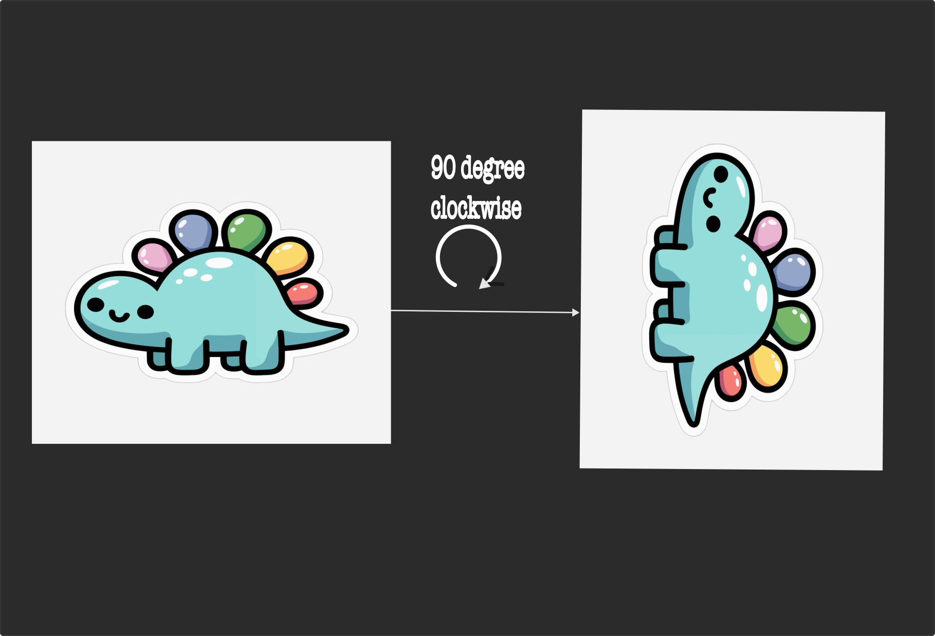
First, we begin with an image of a little dino. Suppose we rotate him by 90 degrees clockwise. The right side of the figure shows the rotated dino. The question we wish to ask is: what might be happening in our heads when we see the rotated dino?

There are two answers:

Nothing happens. Even if it is rotated, it is still a dino.
The brain builds an internal representation of the dino. Let us call it R1. Upon rotation of the dino, the brain computes a new representation, R2. R1 and R2 are related to each other in some predictable way. So the brain then does some sort of computation to see that R1 and R2 are in fact similar.

At first glance, it seems the first one is more desirable. The representation never changes, so there is no need for post-processing. That is called invariance.

The second one seems undesirable. It comes at the cost of defining how the representation in the brain might work, figuring out a bunch of weird math, and then doing all the bookkeeping needed to relate R1 and R2 to each other. That is called equivariance.

If someone asked you, “hey dude, should I choose invariance or equivariance when building my neural net?”, your answer would be: “Geez, build invariance, man. It’s simple, faster, and cheaper to compute.”

The argument for the rest of this post is counterintuitive: equivariance is far better than invariance. However, to understand it, we have to bring in a cute turtle. There are two types of turtle we wish to consider: 1) the arrogant turtle and 2) the humble turtle. Most turtles in this world are arrogant.

The arrogant turtle

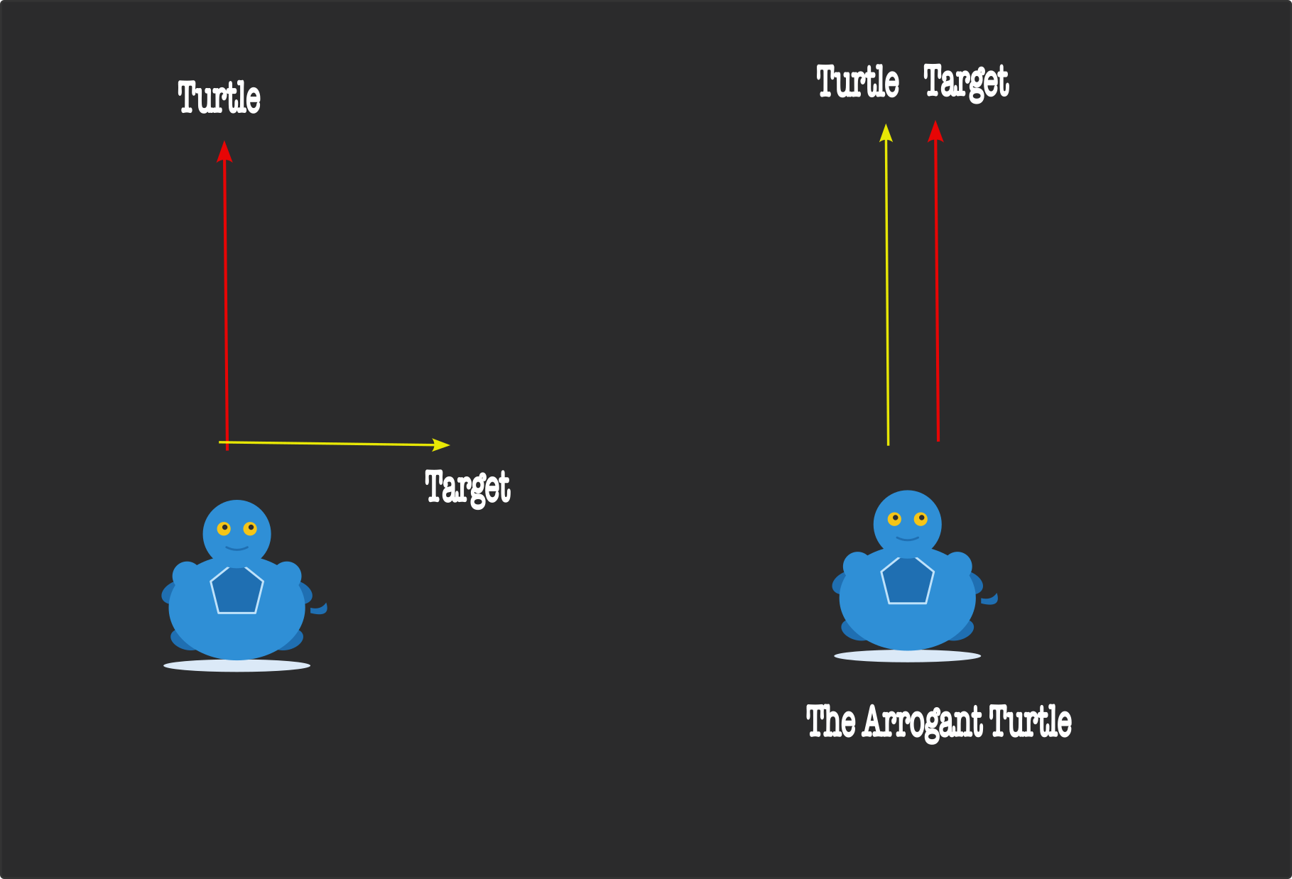
On the left, we show a blue turtle. He is represented by a red vector. There is a target vector (in yellow) perpendicular to him. The target vector sits in the outside world. The blue turtle is the neural net. The task is to align the two arrows (just for the fun of it).

Recall that the turtle is arrogant. He would rather stick to his place and wait for the world to adjust according to him. But this world is big, and the whims of a little turtle do not concern it. For the moment, though, we assume that the world does bend to the whims of the turtle.

The yellow target turns clockwise, and the two vectors align. Both the turtle and the world are now happy.

Let us consider the same case from the opposite perspective.

The humble turtle

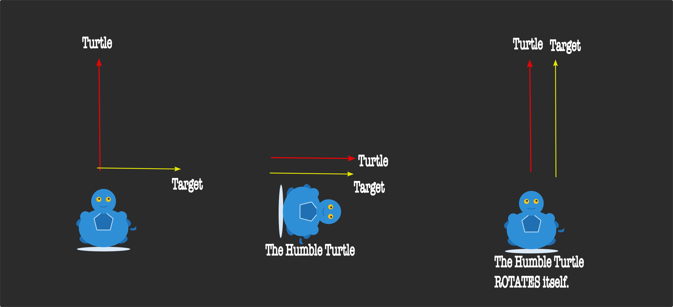
The turtle in the above figure (extreme left) is humble. He knows the world will not bend to his whims. There are just so many turtles in the world. The only option the turtle has is to adjust himself. The turtles who submit themselves to what the world demands of them outlive those that refuse to adjust. Darwin called that survival of the fittest, lol.

So anyway, our turtle (in the middle of the picture) rotates clockwise and aligns himself with the world. They are happy. However, you, dear reader, are not happy. You see both of them rotated now, so you would rather prefer them to be upright. So you tell the turtle: “Dear turtle, can you please rotate yourself to align with me?”

The turtle says: “Sure, master, I am humble, and I will do whatever you say.” So he takes his perception of the world (the yellow vector), along with his own vector (red), and rotates both to align vertically on the screen. Everything looks beautiful once again.

The humble turtle thinks: “Alas, what is beauty? I can feel it, but I have no way of quantifying it. How may I even start to model it?” He makes a note to ask Schmiduber for guidance later. For now, however, the turtle has grown weary. All that rotation and counter-rotation have deeply exhausted his mojo.

Our dear turtle closes his eyes, retreats into his shell, and enters a deep state of trance. Smoking a little cigar always helps. Our turtle then goes into a deep silence, for only then does mother nature reveal her mysteries. The musings of the outer world no longer concern it. The turtle only opens its eyes when it is time to make other turtles by the sea. For some reason, the turtle just lays eggs and continues on its merry way. He does not have to mate for life or pledge its allegiance to a single female turtle forever. Humans, on the other hand, do. Perhaps it is more fun to be a turtle.

The above story leads one to believe that we may have made a mistake of public posturing. However, that might not be correct. One may also believe that we could learn from the humble turtle more than from the arrogant turtle. However, the turtles who are arrogant in the eyes of few are merely committed to their own ways of existing. So we will turn to the arrogant turtle to learn from him.

It is now time to move away from the realm of the mystics and into the realm of engineering.

Lessons from the arrogant turtle

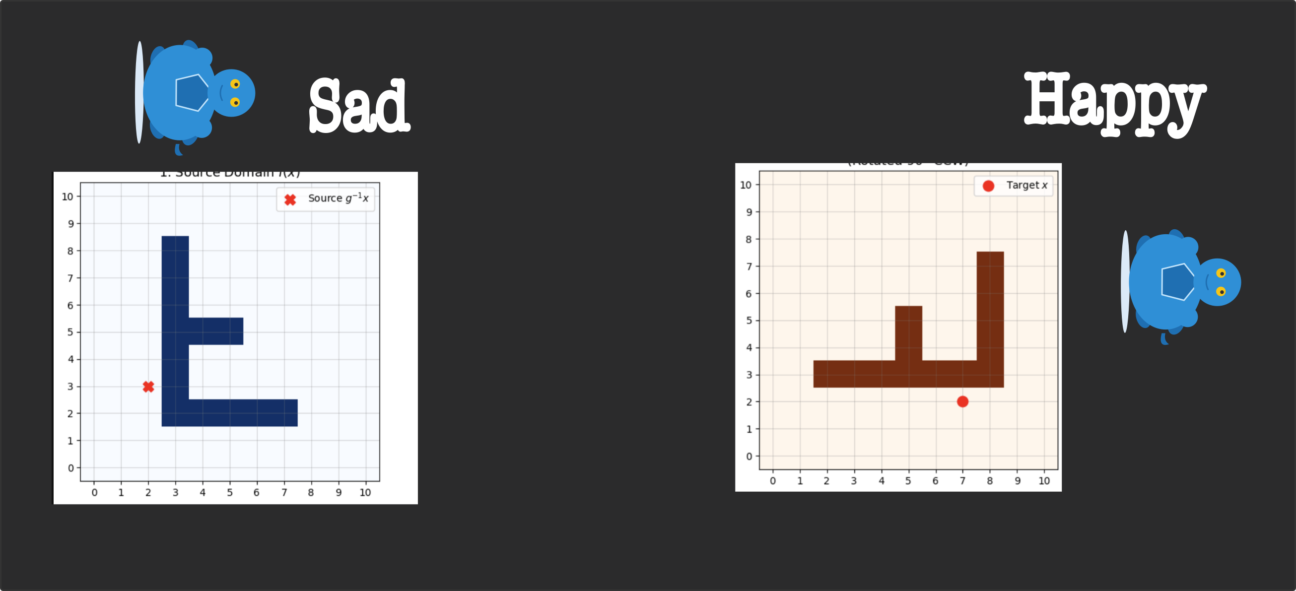
We would now like to think of our turtle as a kernel of a convolutional net. The picture above shows a rotated (and inverted) image of a letter F. The kernel can either be sad or happy in this case. The left part of the picture shows the turtle as sad. This is because the turtle does not align with the larger horizontal line on the F. In the right picture, the image has been rotated clockwise. The turtle now begins to face the latter F (the upper line in the F), so it is happy.

Now, let us consider the matter of how we actually rotate an image in a computer. First, let me dump some code I wrote, and then explain what it means.

import matplotlib.pyplot as plt
import numpy as np

# 1. Create a dummy feature map f(x) with an asymmetrical pattern (an 'F')
N = 11  # Grid size (11x11, centered at origin (0,0))
f = np.zeros((N, N))

# Draw an "F" pattern on the grid
f[2:9, 3] = 1.0  # Vertical stem
f[2, 3:8] = 1.0  # Top bar
f[5, 3:6] = 1.0  # Middle bar

# 2. Define grid coordinates centered at (0, 0)
coords = np.stack(
    np.meshgrid(np.arange(N) - N // 2, np.arange(N) - N // 2), axis=-1
)

# 3. Define transformation g: 90-degree counter-clockwise rotation matrix
R_g = np.array([[0, -1], [1, 0]])
R_g_inv = R_g.T

# 4. Compute [L_g f](x) = f(g^{-1}x)
L_g_f = np.zeros((N, N))

for i in range(N):
    for j in range(N):
        x = coords[i, j]  # Target coordinate [x_1, x_2]
        x_src = R_g_inv @ x  # Inverse lookup: g^{-1} x

        src_i, src_j = x_src[1] + N // 2, x_src[0] + N // 2

        if 0 <= src_i < N and 0 <= src_j < N:
            L_g_f[i, j] = f[src_i, src_j]

# 5. Plotting: Original f(x) -> Forward Mapping -> Transformed [L_g f](x)
fig, axes = plt.subplots(1, 3, figsize=(16, 5))

# --- Panel 1: Source Domain f(x) ---
axes[0].imshow(f, cmap="Blues", origin="lower")
axes[0].set_title(r"1. Source Domain $f(x)$", fontsize=13)
axes[0].set_xticks(np.arange(N))
axes[0].set_yticks(np.arange(N))
axes[0].grid(True, color="gray", alpha=0.3)

# --- Panel 2: Coordinate Mapping (Forward Vectors) ---
axes[1].imshow(f, cmap="Blues", alpha=0.25, origin="lower")
axes[1].set_title(
    r"2. Forward Mapping: $x_{\text{dest}} = g \cdot x_{\text{src}}$", fontsize=13
)
axes[1].set_xticks(np.arange(N))
axes[1].set_yticks(np.arange(N))
axes[1].grid(True, color="gray", alpha=0.3)

# Overlay vector field showing where non-zero points in f(x) move to under g
for i in range(N):
    for j in range(N):
        if f[i, j] > 0:
            # Source coordinate (x, y) centered at origin
            x_src = np.array([j - N // 2, i - N // 2])

            # Forward coordinate transformation: x_dest = g * x_src
            x_dest = R_g @ x_src

            # Convert to array plotting indices
            src_col, src_row = j, i
            dest_col, dest_row = x_dest[0] + N // 2, x_dest[1] + N // 2

            # Compute displacement vector (dx, dy)
            dx = dest_col - src_col
            dy = dest_row - src_row

            # Draw mapping arrow from source to destination
            axes[1].quiver(
                src_col,
                src_row,
                dx,
                dy,
                angles="xy",
                scale_units="xy",
                scale=1,
                color="darkorange",
                alpha=0.8,
                width=0.015,
                headwidth=4,
            )

# --- Panel 3: Destination Domain [L_g f](x) ---
axes[2].imshow(L_g_f, cmap="Oranges", origin="lower")
axes[2].set_title(
    r"3. Destination Domain $[L_g f](x)$" + "\n(Rotated 90° CCW)", fontsize=13
)
axes[2].set_xticks(np.arange(N))
axes[2].set_yticks(np.arange(N))
axes[2].grid(True, color="gray", alpha=0.3)

# Highlight single point pair across all three subplots
target_x, target_y = 2, -3  # Target point in L_g_f
target_i, target_j = target_y + N // 2, target_x + N // 2

src_coords = R_g_inv @ np.array([target_x, target_y])
src_i, src_j = src_coords[1] + N // 2, src_coords[0] + N // 2

axes[0].scatter(
    src_j,
    src_i,
    color="red",
    s=110,
    zorder=5,
    label=r"Source $g^{-1}x$",
    marker="X",
)
axes[1].scatter(
    src_j, src_i, color="red", s=110, zorder=5, marker="X", label=r"Source"
)
axes[1].scatter(
    target_j, target_i, color="red", s=110, zorder=5, label=r"Destination"
)
axes[2].scatter(
    target_j, target_i, color="red", s=110, zorder=5, label=r"Target $x$"
)

axes[0].legend(loc="upper right")
axes[1].legend(loc="upper right")
axes[2].legend(loc="upper right")

plt.tight_layout()
plt.show()

Rather than look at all the mess, just look at the picture below:

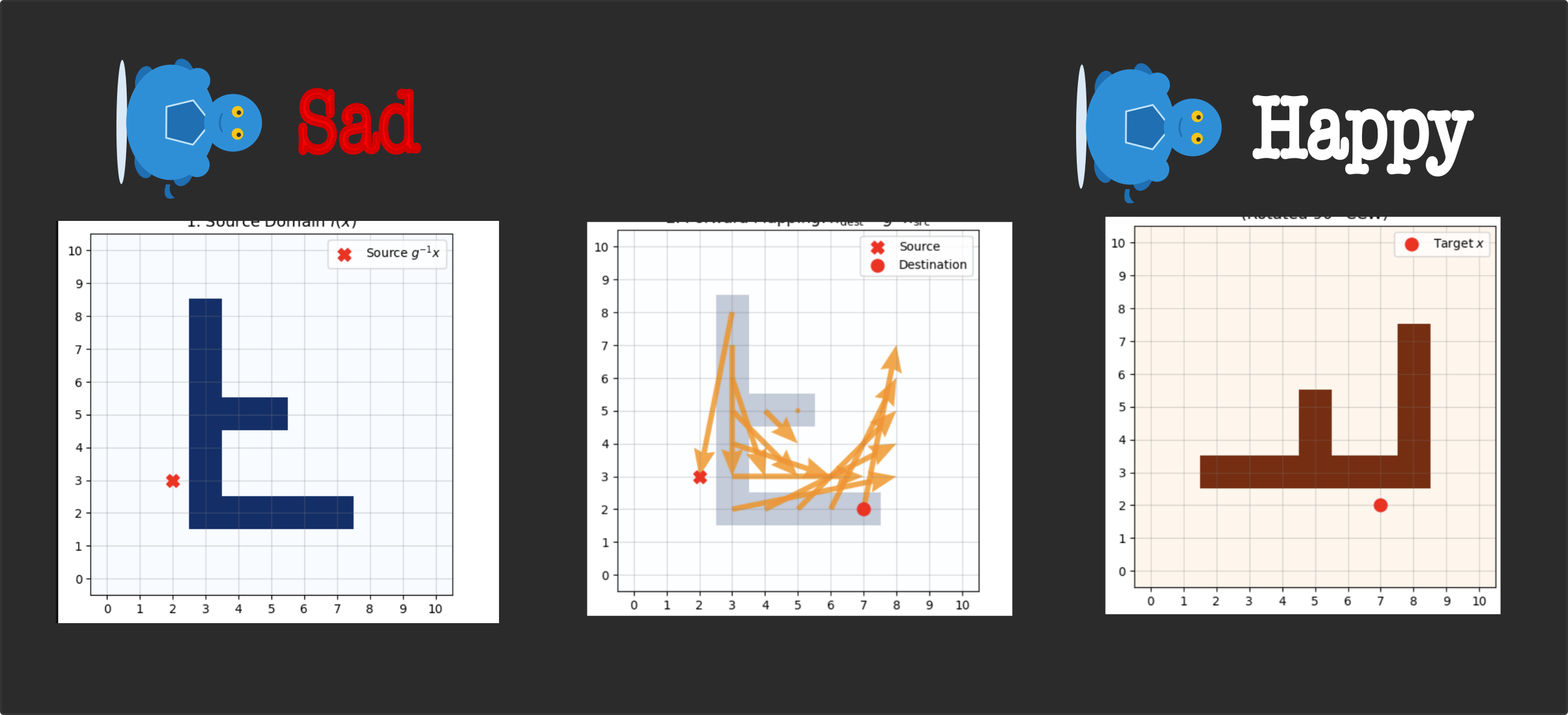
The middle panel shows, by means of arrows, which source point in the original image goes to which destination point of the final image. That is all the above code is trying to achieve. Specifically, the code begins by defining a rotation matrix R. When this rotation matrix acts on any src point $(x, y)$, it transforms it into a new dest point. One other way to do it is as follows:

for i in range(N):
    for j in range(N):
        x = coords[i, j]  # Target coordinate [x_1, x_2]
        x_src = R_g_inv @ x  # Inverse lookup: g^{-1} x

        src_i, src_j = x_src[1] + N // 2, x_src[0] + N // 2

        if 0 <= src_i < N and 0 <= src_j < N:
            L_g_f[i, j] = f[src_i, src_j]

You draw a single canvas called L_g_f. Then you go through each row and each column, and choose a point. Let us call it dest. You ask: “Dear dest, which source value should I fill you with?” You can get that x_src by applying the operation R_g_inv @ x. Here, x is the coordinate on the dest grid, not the src grid. Once you make sure that the src point actually lies within the bounds of your grid, you can replace it with the value.

What is the point of this entire exercise? Two things stand out:

If a src image has to be rotated by 90 degrees clockwise, we can precompute a dictionary mapping every src point to its corresponding dest point. The contents of this dictionary never change.
The mapping stored in this dictionary does not depend on what is actually drawn on it. No matter what content there is, the same dictionary will hold true.
An action of this dictionary is the physical act of creating a dest canvas and manually copying the pixels from src to dest.
Now let us assume that the image is to be rotated three times clockwise. We can merely perform the action of applying the dictionary to the image three times one after another.

In a sense, the mapping that the dictionary holds is the representation of the potential act of rotating the image by multiples of 90 degrees. For two-dimensional images, there are 4 possible rotations: 90, 180, 270, and 360 degrees. A full rotation of 360 degrees recovers the original image without any loss of information.

So let us start from 0 and want to get to 270. We need three rotations: 0 → 90 → 180 → 270. Is it possible to get directly to 270? Perhaps. But we will assume that reaching 270 still requires the repeated action of the dictionary. Why? It seems nonsense. To go from 0 to 270, it is possible to multiply the dictionary D three times as D·D·D and apply the resultant operator directly to the input image. This is far faster than doing D, DD, and DDD one after another. That makes no sense.

Well, my dear reader, the fact that you can just apply D three times recursively, even if it takes longer, is of interest because compute is cheap while memory is not: it is easier to store D than to store the three separate operators D, DD, and DDD together. So let us make this assumption for now. Those of us in the GLOM business now call this D a geometric operator. It might be hardcoded, or it might be a super cute learned mapping for transforming input (like Hinton’s transforming autoencoder, hehe).

Now, we will start asking ourselves a few stupid questions and gradually build towards a more general solution.

Q1. Suppose we want to build a neural net that can detect 90-degree rotations of an object. How do we build one?

Answer: Indeed, when we used only one turtle, it was able to detect only one rotation. A group of 90-degree rotations contains 4 possible rotations: 90, 180, 270, and 360 degrees. So perhaps we need 4 possible turtles. We are therefore tempted to invent a generic data structure of turtles called a filter bank.

Here is how it may look:

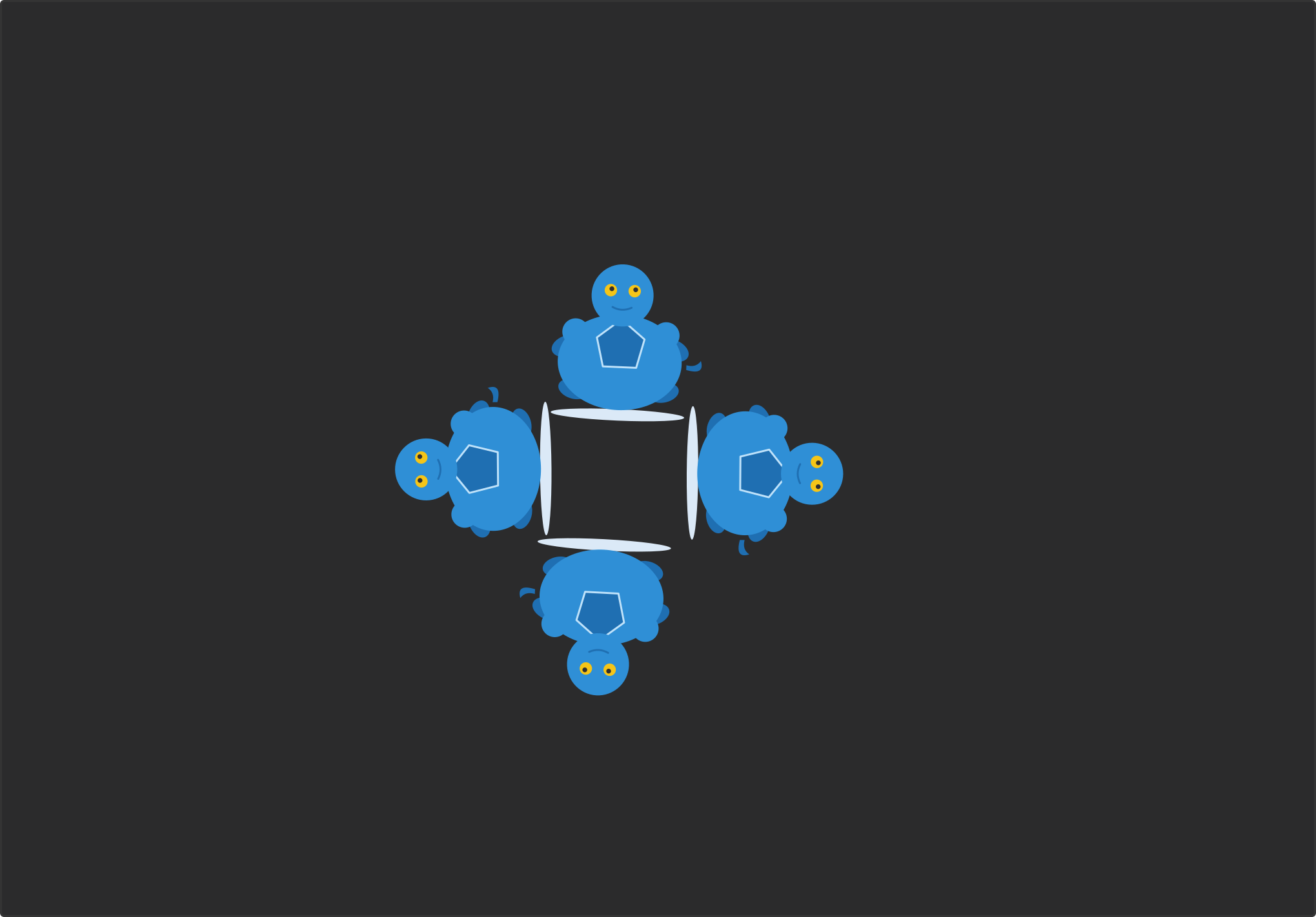
The above filter bank contains 4 turtles (4 filters) arranged in a nice fashion. Now, let us imagine that we are one of the turtles. In other words, we are a CNN filter. Now, an image in the outside world can undergo 4 rotations. We want to study how the `combined set’ of filter banks will respond to the changing images. A pictorial description is provided below:

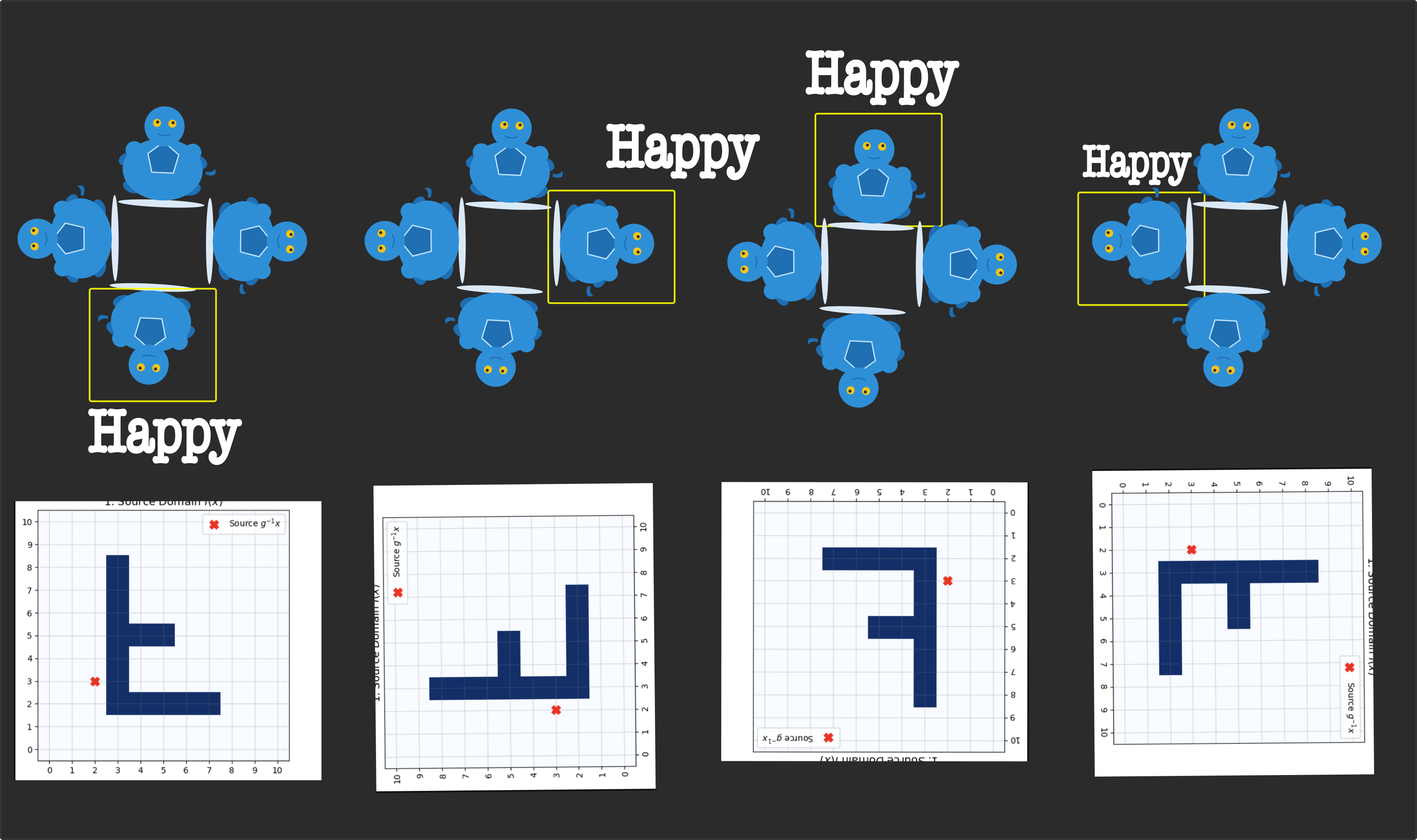
A yellow rectangle in the filter bank shows which of the turtles gets activated. As you can see, the yellow box undergoes an anticlockwise rotation. This leads us to two very subtle points:

Case 1: If the world outside changes anticlockwise, the pattern of responses in a filter bank also triggers anticlockwise over time.
Case 2: Now suppose the world outside does not change. The image being fed to the network is of a single orientation (for example, the leftmost image of the inverted letter F). We still want to achieve a similar pattern of activity to the one triggered by the actual rotation of the letter F in the previous case. This mental act of simulating an actual rotation of the world inside the neural net itself is what is termed mental rotation (Shephard).

We must understand a few more subtleties of case 1 and case 2. The representation R produced in both cases is the same. It is the fundamental nature of computation that has now changed.

In case 1, the world rotated, so the input was fed 4 times to the network (for the 0°, 90°, 180°, and 270° rotations). In the second case, the input was fed only once, but the mental rotation happened for the 4 filters in parallel. Case 1 consumes more compute since the data may have to travel through the network 4 times. On the other hand, case 2 consumes less compute. I will come back to this later, but for now let us stay on track. Please email me if I forget to cover this here.

Thus, it has now become really tempting to use case 2: after all, it uses less compute and gives the same answer, so why not use it, lol? However, as they say, good things in life do not come free. Everything comes at a cost. You must be willing to pay it. Even if you are not, a transformer architecture is extracting it from you.

The cost of mental rotation

Let us recall our filter bank from earlier:

It contains 4 separate filters (or turtles). However, this sort of representation creates several issues:

There is a separate filter for each orientation we wish to detect. For example, if 4 rotations are to be made, there will be 4 filters. Let us assume we now wish to change the precision of the rotations we detect. For example, we want to be able to encode equivariance at every multiple of 10 degrees. So we would have a filter for 10, 20, 30, …, 360 degrees, for a total of 36 filters. Hence, the number of filters has shot up from 4 to 36.
This means that the representation is stupid: it scales linearly with the precision of rotation. It means that to encode rotation equivariance at infinite precision, an infinite number of parameters would be required. Surely, the brain does not do that. (Disclaimer: to be honest, we do not know what the brain does. People sorta model how it might work, build a way to test it in a computer, and if the results are good, call it a day. But the brain does not care about state of the art; it might care about efficiency, though, since there is only so much energy you can extract from a human cell, lol.)

What then is the answer? Two words: weight sharing.

The phenomenon of mental rotation suggests us a curious fact: rather than storing 4 separate filters, it must be possible to copy a single filter at 4 different orientations to create 4 separate filters. Each filter then responds to a different orientation of the image, and hence creates its own pattern of neural activity. This is called weight sharing of a filter across orientations.

Till now, we merely talked about rotations. What about translations? Let us now start with another analogy:

Suppose you are a vector. You have two choices. Either you can rotate. Or you can translate. If you choose to rotate, you rotate at multiples of 90. If you translate, you can translate by any amount.

Together, the combination of rotation and translation could be represented by a single rotation matrix $R$. There is one more issue:

Let us assume you rotate first, and then translate. Alternatively, you translate first and rotate then. In both cases, do you end up at the same destination (a.ka. a point in the subspace)?

The answer is a whopping no. This leads one to believe that the order of application of rotation, translation should be encoded in the weights of a neural net. However, what mathematicians call as commutativity need not hold for neural nets. Let me explain.

Suppose you perform two actions called rotation $R$ and translation $t$. There are two possible paths $R \rightarrow t$, $t \rightarrow R$. If you choose to pack $<R, t>$ together in a single rotation matrix, then it sort of guarantees a curious thing: no matter the path you take, there will be one unique rotation matrix which encodes that action. The job of the neural net then is just to find it in the higher dimensional space.

The key takeaway is: it is possible to make a copy of a SINGLE filter, and store those filter at different orientations. Those filters can then operate in parallel to produce a distributed pattern of neural activity. Let us first implement this.

import numpy as np
import matplotlib.pyplot as plt

rng = np.random.default_rng(0)
psi = rng.normal(size=(5,5))        # our stencil -- 25 random numbers in a 5x5 grid

def rot(a, k):
    return np.rot90(a, k)           # rotates array `a` by 90 degrees, k times

fig, axes = plt.subplots(1, 4, figsize=(13,3.6))
for g, ax in enumerate(axes):
    im = ax.imshow(rot(psi, g), cmap='coolwarm', vmin=-2, vmax=2)
    ax.set_title(f"rot(psi, {g})\n({g*90} degrees)", fontsize=10)
    ax.axis('off')
plt.tight_layout(); plt.show()

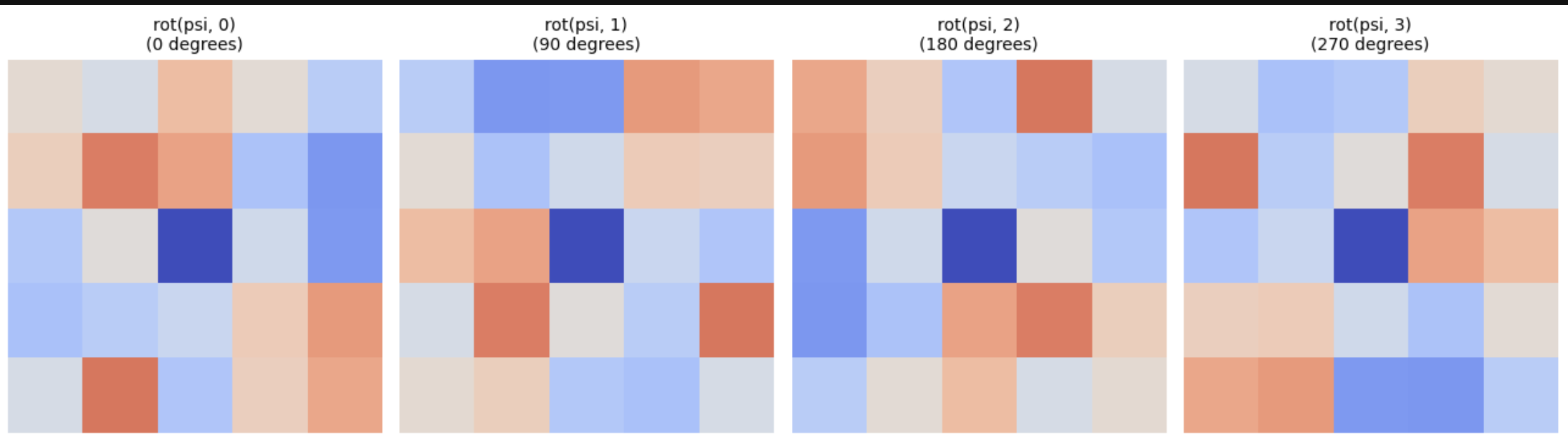
So, we start with a kernel of 5 by 5. The values inside the kernel are not important: they will be learned. However, the idea that the kernel is rotated 4 times and produces 4 sets of neural activations is of great interest. Let us now focus on this matter. Above, you can see what the kernel looks like after it rotates 4 times. Note that we do not seek symmetry in the weights of the kernel itself; however, we do seek symmetry in the action of the kernel, i.e. in its rotations by 90 degrees.

The tensor tracking

Let us now imagine that we are given an image of size $(B, 3, H, W)$. We wish to define a kernel on it of size $3, d, d, C_{out}$. Assume there will be $N$ such kernels. For now, we shall focus on a single kernel. Let us try to track the input tensor from the perspective of one such kernel.

The kernel will create 4 copies. Each copy will create a neural pattern of dimension $B, C_{out}, H, W$. There are 4 such kernels, so their output will be stacked along a new axis. So the output tensor now starts looking like $B, C_{out}, 4, H, W$, where 4 is the number of stored rotations of the kernel.

Generalizing this, there are $N$ such kernels, so there will be another $N$ such tensors stacked together. Therefore, the output is now $B, N, 4, H, W$, where $N \times 4 = C_{out}$. Easy peasy. Hiyaaa!!

The operation above is restricted to the first layer of the network, which lifts an input image of 3 dimensions into higher ones. However, let us first build it concretely.

import numpy as np
from scipy.signal import correlate2d

rng = np.random.default_rng(0)

B, C_in, H, W = 2, 3, 16, 16
N, d = 5, 5

# INTEGER-valued data -- small whole numbers, exactly representable in float64
x = rng.integers(-3, 4, size=(B, C_in, H, W)).astype(np.float64)
kernels = rng.integers(-3, 4, size=(N, C_in, d, d)).astype(np.float64)

def rot(a, k):
    return np.rot90(a, k, axes=(-2,-1))

def corr2d(img, k):
    return correlate2d(img, k, mode='same', boundary='fill', fillvalue=0)

def lift_layer1(x, kernels):
    B, C_in, H, W = x.shape
    N, _, d, _ = kernels.shape
    out = np.zeros((B, N, 4, H, W))
    for g in range(4):
        rotated_kernels = rot(kernels, g)
        for b in range(B):
            for n in range(N):
                acc = np.zeros((H, W))
                for c in range(C_in):
                    acc += corr2d(x[b, c], rotated_kernels[n, c])
                out[b, n, g] = acc
    return out

def Lg_stack_batched(f_stack, r):
    return np.stack([rot(f_stack[:, :, (g - r) % 4], r) for g in range(4)], axis=2)

O_original = lift_layer1(x, kernels)
r = 1
x_rotated = rot(x, r)
O_from_rotated_input = lift_layer1(x_rotated, kernels)
O_undone = Lg_stack_batched(O_from_rotated_input, -r)

error = np.abs(O_undone - O_original).max()
print("error:", error, "  exactly zero?", error == 0.0)

output: error: 0.0 exactly zero? True

What we are basically doing is that we create some data and run it through the group-equivariant layer first. Next, we rotate the input by 90 degrees and run it through the equivariance net again. Then we rotate the output in the opposite 90-degree direction. The two answers should match and be exactly 0. If so, then the net is said to have encoded equivariance. Please note the following line: x = rng.integers(-3, 4, size=(B, C_in, H, W)).astype(np.float64). What this is saying is that the data in the input should be perfectly integer-valued for the perfect 0 loss to hold. If it is a float, there will be some error that accumulates, and the representation does not hold perfectly equivariant anymore.

Folks in the ML community get away with this issue: a little error is okay, as long as some symmetry is being baked into the architecture. While this solves the problem, there is an issue: if you want your neural net to be precise—absolutely precise—it will not work. The difference, while subtle, stacks up: you can no longer break encryptions using neural nets, since the errors compound. A better design might help get rid of this issue.

Simulating the mental rotation

You might have noticed a subtle issue: to test for equivariance, I had to run the original image and the rotated version of it through the net. Is it possible to perform something equivalent to the physical rotation of the input inside the representation of the neural net itself? If so, then it is called mental rotation. Turns out, there is. Time to dump some more code, lol.

import numpy as np
from scipy.signal import correlate2d

rng = np.random.default_rng(0)
B, C_in, H, W = 2, 3, 16, 16
N, d = 5, 5

x = rng.integers(-3, 4, size=(B, C_in, H, W)).astype(np.float64)
kernels = rng.integers(-3, 4, size=(N, C_in, d, d)).astype(np.float64)

def rot(a, k):
    return np.rot90(a, k, axes=(-2,-1))

def corr2d(img, k):
    return correlate2d(img, k, mode='same', boundary='fill', fillvalue=0)

def lift_layer1(x, kernels):
    B, C_in, H, W = x.shape
    N, _, d, _ = kernels.shape
    out = np.zeros((B, N, 4, H, W))
    for g in range(4):
        rotated_kernels = rot(kernels, g)
        for b in range(B):
            for n in range(N):
                acc = np.zeros((H, W))
                for c in range(C_in):
                    acc += corr2d(x[b, c], rotated_kernels[n, c])
                out[b, n, g] = acc
    return out

O_original = lift_layer1(x, kernels)    # (B,N,4,H,W) -- from the UNROTATED input
r = 1
O_physical = lift_layer1(rot(x, r), kernels)   # (B,N,4,H,W) -- ground truth, from the ROTATED input

# --- pool away the spatial axes entirely -- 'store the responses', no H,W left to worry about ---
pooled_original = O_original.sum(axis=(-2,-1))         # (B, N, 4)
pooled_physical  = O_physical.sum(axis=(-2,-1))          # (B, N, 4)
print("pooled shape:", pooled_original.shape)

# --- mental rotation: PURE axis permutation on the pooled vector, nothing spatial left to rotate ---
def mental_rotate_pooled(pooled, r):
    idx = [(g - r) % 4 for g in range(4)]
    return pooled[:, :, idx]

pooled_mental = mental_rotate_pooled(pooled_original, r)

error = np.abs(pooled_mental - pooled_physical).max()
print("mental-rotation-via-pure-axis-permutation error (on POOLED activity):", error)

Note the subtlety here: we started from the original image and then simulated the mental rotation of 90 degrees by shifting the neural activity along the axis of the filter axis. This only held when the intermediate feature map of $B, N, 4, H, W$ was spatially pooled to $B, N, 4$, i.e. when we lost the spatial information altogether. It might be helpful to draw a picture of this:

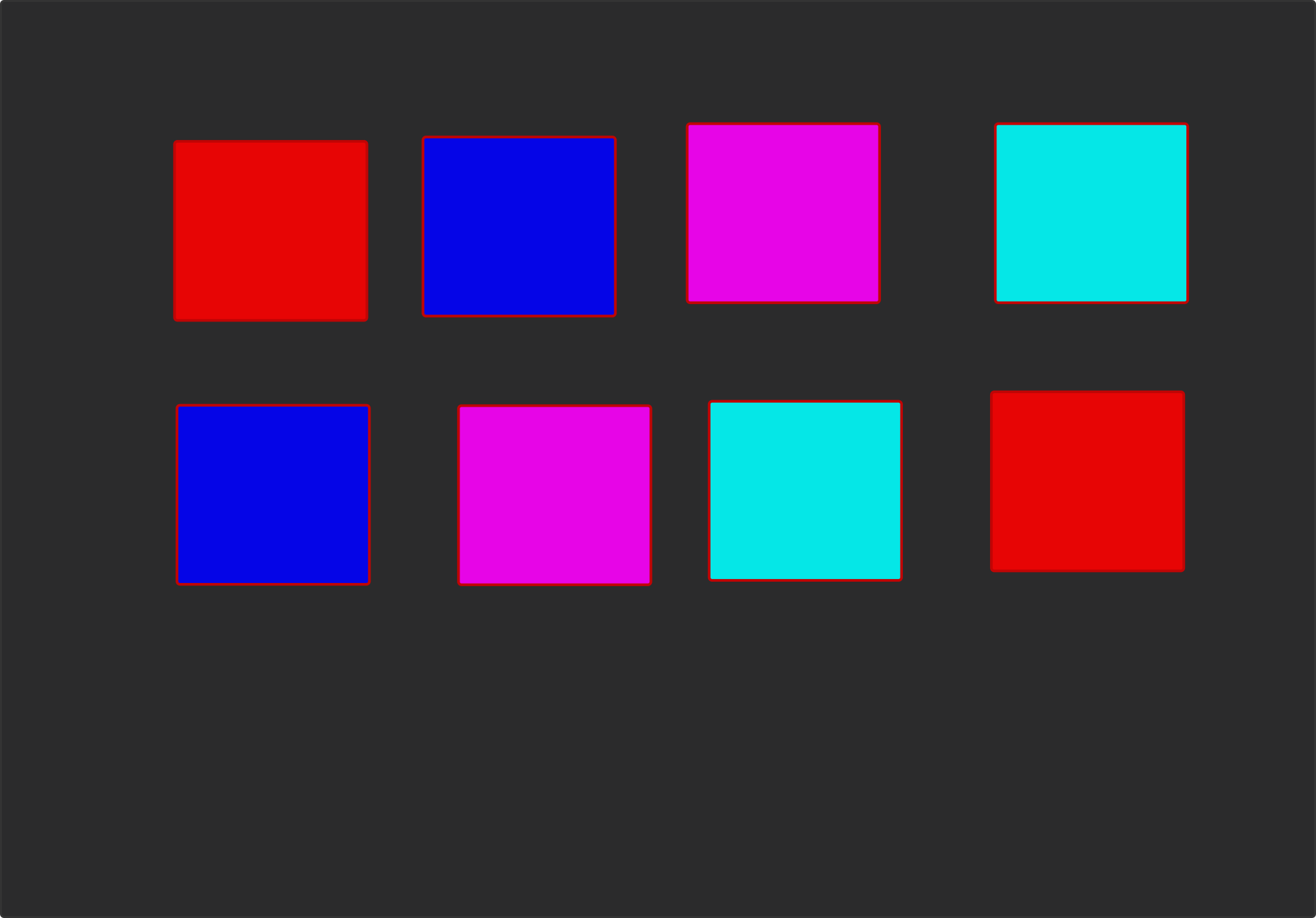
The key idea is as follows: look at the first row. Different colors represent different responses of the internal filters in the neural net. If you want to simulate the actual rotation of the object, you can just shift the responses along the axis. For example, the blue square in the first row moves to the left and becomes the first square in the second row. Notice the wraparound: the red neural activity (in the first row) wraps around to become the last square in the second row. This is what the following lines are doing, lol:

def mental_rotate_pooled(pooled, r):
    idx = [(g - r) % 4 for g in range(4)]
    return pooled[:, :, idx]

Now, let us consider the matter of the loss of spatial information when the actual convolution is performed prior to pooling. Suppose you are given two integers, $2$ and $3$. There are two ways to add them: either $2 + 3$ or $3 + 2$. If I gave you the answer $5$ and asked which order of numbers you used to add them, you would not know, lol. Or you might say, “You know what, it is $2+3$ with 50% probability and $3+2$ with 50% probability.” The key point is that there is no way to encode the order of operation, i.e. the physical locations of the variables $2$ and $3$ themselves (there are two slots for addition, so which number maps to which) within the convolution operation itself. It collapses the signal and loses useful information. Therefore, convolution makes no sense. However, for the rest of this (shit) post, we will assume convolution is all we know. (Personally, however, I like neither convolution nor attention; maybe it is time for something new, lol.) Anyway, let us continue with the matter at hand.

Now let us recall where we actually stand:- We have built a layer which can take an input of $(B, 3, H, W ) $ and lift it to $(B, N, 4, H , W)$. The next order of the business is to build a general layer which can operate from second layer onwards in the neural net. More precisely, we need a layer of the following properties:

Layer 2-onward: parameters for the general group-correlation layer

Input: (B, N_in, 4, H, W) — the output of the previous layer
- B = batch size
- N_in = number of feature channels carried forward from the previous layer
- 4 = the orientation axis (fixed by the group $C_4$)
- H, W = spatial dimensions
Kernel: (N_out, N_in, 4, d, d) — critically, the kernel itself now needs a 4-sized group axis too
- N_out = number of output feature channels this layer produces
- N_in = must match the input’s N_in (summed over)
- 4 = the kernel’s own orientation axis
- d, d = spatial kernel size
Output: (B, N_out, 4, H, W) — same shape family as the input (batch, channels, orientation-axis-of-size-4, spatial), so this layer can be stacked on top of itself arbitrarily many times

Building the second layer

import numpy as np
from scipy.signal import correlate2d

# =============================================================================
# SHARED HELPERS
# =============================================================================

def rot(a, k):
    return np.rot90(a, k, axes=(-2, -1))

def corr2d(img, k):
    return correlate2d(img, k, mode='same', boundary='fill', fillvalue=0)

def Lg_stack(f_stack, r):
    """Rotate a (..., 4, H, W) G-feature map: cyclic-shift the orientation axis
    (assumed to be axis=-3) AND spatially rotate."""
    return np.stack([rot(f_stack[..., (g - r) % 4, :, :], r) for g in range(4)], axis=-3)

# =============================================================================
# LAYER 1: Z^2 -> G      (B, C_in, H, W) -> (B, N, 4, H, W)
# =============================================================================

def lift_layer1(x, kernels):
    """x: (B, C_in, H, W)   kernels: (N, C_in, d, d)   ->   (B, N, 4, H, W)"""
    B, C_in, H, W = x.shape
    N, _, d, _ = kernels.shape
    out = np.zeros((B, N, 4, H, W))
    for g in range(4):
        rotated_kernels = rot(kernels, g)
        for b in range(B):
            for n in range(N):
                acc = np.zeros((H, W))
                for c in range(C_in):
                    acc += corr2d(x[b, c], rotated_kernels[n, c])
                out[b, n, g] = acc
    return out

# =============================================================================
# LAYER 2+: G -> G       (B, N_in, 4, H, W) -> (B, N_out, 4, H, W)
# =============================================================================

def group_corr_layer(f_stack, kernels):
    """
    f_stack: (B, N_in, 4, H, W)        -- output of a previous G-CNN layer
    kernels: (N_out, N_in, 4, d, d)    -- the kernel ITSELF now has a group axis
    returns: (B, N_out, 4, H, W)
    """
    B, N_in, G, H, W = f_stack.shape
    N_out, N_in_k, G_k, d, _ = kernels.shape
    assert N_in == N_in_k, f"N_in mismatch: input has {N_in}, kernel expects {N_in_k}"
    assert G == G_k == 4, "this implementation is specialized to the C4 group (size 4)"

    out = np.zeros((B, N_out, 4, H, W))
    for g_out in range(4):
        for g_in in range(4):
            s = (g_in - g_out) % 4                       # the group-multiplication rule (eq 11)
            rotated_kernel_slice = rot(kernels[:, :, s], g_out)   # (N_out, N_in, d, d)
            for b in range(B):
                for n_out in range(N_out):
                    for n_in in range(N_in):
                        out[b, n_out, g_out] += corr2d(f_stack[b, n_in, g_in],
                                                        rotated_kernel_slice[n_out, n_in])
    return out

rng = np.random.default_rng(0)
PASS, FAIL = [], []

def check(name, condition):
    (PASS if condition else FAIL).append(name)
    print(("[PASS] " if condition else "[FAIL] ") + name)

print("="*70)
print("TEST SUITE: group_corr_layer")
print("="*70)

# -----------------------------------------------------------------------
# TEST 1: shape correctness
# -----------------------------------------------------------------------
print("\n--- Test 1: output shape ---")
B, N_in, H, W = 2, 4, 14, 14
N_out, d = 6, 3
f_stack = rng.normal(size=(B, N_in, 4, H, W))
kernels = rng.normal(size=(N_out, N_in, 4, d, d))

out = group_corr_layer(f_stack, kernels)
expected_shape = (B, N_out, 4, H, W)
check(f"output shape is {expected_shape}", out.shape == expected_shape)

# -----------------------------------------------------------------------
# TEST 2: floating-point equivariance (round-trip: rotate in, undo on the way out)
# -----------------------------------------------------------------------
print("\n--- Test 2: floating-point equivariance (round-trip) ---")
r = 1
f_rotated = Lg_stack(f_stack, r)
out_from_rotated = group_corr_layer(f_rotated, kernels)
out_undone = Lg_stack(out_from_rotated, -r)

err_float = np.abs(out_undone - out).max()
print(f"    max error: {err_float:.2e}")
check("floating-point round-trip error is tiny (< 1e-8)", err_float < 1e-8)

# -----------------------------------------------------------------------
# TEST 3: exact-zero equivariance with integer data
# -----------------------------------------------------------------------
print("\n--- Test 3: EXACT (integer-valued) equivariance ---")
f_stack_int = rng.integers(-3, 4, size=(B, N_in, 4, H, W)).astype(np.float64)
kernels_int = rng.integers(-3, 4, size=(N_out, N_in, 4, d, d)).astype(np.float64)

out_int = group_corr_layer(f_stack_int, kernels_int)
f_rot_int = Lg_stack(f_stack_int, r)
out_from_rot_int = group_corr_layer(f_rot_int, kernels_int)
out_undone_int = Lg_stack(out_from_rot_int, -r)

err_int = np.abs(out_undone_int - out_int).max()
print(f"    max error: {err_int}")
check("integer round-trip error is EXACTLY 0.0", err_int == 0.0)

# -----------------------------------------------------------------------
# TEST 4: all four rotations (not just r=1), integer data
# -----------------------------------------------------------------------
print("\n--- Test 4: all 4 rotations individually ---")
for rr in range(4):
    f_rot = Lg_stack(f_stack_int, rr)
    out_rot = group_corr_layer(f_rot, kernels_int)
    predicted = Lg_stack(out_int, rr)
    e = np.abs(out_rot - predicted).max()
    check(f"r={rr}: exact equivariance (error == 0.0)", e == 0.0)

# -----------------------------------------------------------------------
# TEST 5: identity rotation (r=0) should be a no-op
# -----------------------------------------------------------------------
print("\n--- Test 5: r=0 is a no-op ---")
check("Lg_stack with r=0 is the identity", np.array_equal(Lg_stack(f_stack_int, 0), f_stack_int))

# -----------------------------------------------------------------------
# TEST 6: end-to-end composition -- lift_layer1 THEN group_corr_layer, full pipeline
# -----------------------------------------------------------------------
print("\n--- Test 6: end-to-end, lift_layer1 -> group_corr_layer ---")
B2, C_in, H2, W2 = 2, 3, 14, 14
N1, d1 = 4, 3
N2, d2 = 5, 3

x_int = rng.integers(-3, 4, size=(B2, C_in, H2, W2)).astype(np.float64)
k1_int = rng.integers(-3, 4, size=(N1, C_in, d1, d1)).astype(np.float64)
k2_int = rng.integers(-3, 4, size=(N2, N1, 4, d2, d2)).astype(np.float64)

def full_pipeline(x, k1, k2):
    layer1_out = lift_layer1(x, k1)
    layer2_out = group_corr_layer(layer1_out, k2)
    return layer2_out

pipeline_out = full_pipeline(x_int, k1_int, k2_int)
print("    pipeline output shape:", pipeline_out.shape)
check("pipeline output shape is (B, N2, 4, H, W)", pipeline_out.shape == (B2, N2, 4, H2, W2))

r = 1
x_rot = rot(x_int, r)
pipeline_out_from_rot = full_pipeline(x_rot, k1_int, k2_int)
pipeline_undone = Lg_stack(pipeline_out_from_rot, -r)

err_pipeline = np.abs(pipeline_undone - pipeline_out).max()
print(f"    end-to-end round-trip error: {err_pipeline}")
check("end-to-end (2-layer) equivariance is EXACT (0.0)", err_pipeline == 0.0)

# -----------------------------------------------------------------------
# TEST 7: broken baseline -- confirm the test suite can actually catch bugs
# -----------------------------------------------------------------------
print("\n--- Test 7: sanity check -- does a BROKEN layer actually fail these tests? ---")
def broken_group_corr_layer(f_stack, kernels):
    """Deliberately wrong: uses s = (g_in + g_out) % 4 instead of (g_in - g_out) % 4"""
    B, N_in, G, H, W = f_stack.shape
    N_out, N_in_k, G_k, d, _ = kernels.shape
    out = np.zeros((B, N_out, 4, H, W))
    for g_out in range(4):
        for g_in in range(4):
            s = (g_in + g_out) % 4     # <-- BUG: should be minus, not plus
            rotated_kernel_slice = rot(kernels[:, :, s], g_out)
            for b in range(B):
                for n_out in range(N_out):
                    for n_in in range(N_in):
                        out[b, n_out, g_out] += corr2d(f_stack[b, n_in, g_in],
                                                        rotated_kernel_slice[n_out, n_in])
    return out

out_broken = broken_group_corr_layer(f_stack_int, kernels_int)
f_rot_b = Lg_stack(f_stack_int, r)
out_from_rot_b = broken_group_corr_layer(f_rot_b, kernels_int)
out_undone_b = Lg_stack(out_from_rot_b, -r)
err_broken = np.abs(out_undone_b - out_broken).max()
print(f"    broken-layer error: {err_broken}")
check("broken layer correctly FAILS the equivariance test (error > 0)", err_broken > 0)

# -----------------------------------------------------------------------
print("\n" + "="*70)
print(f"SUMMARY: {len(PASS)} passed, {len(FAIL)} failed")
if FAIL:
    print("FAILED:", FAIL)
print("="*70)

The tests pass, so I am somewhat happy.

Now, it is time to take care of the last layer.

Taking care of the last layer

“The fact that pooling works so well is a disaster,” — Geoff Hinton.

We can stack several layers together, as in the last section. Then we have a final feature dimension of $B, N_{out}, 4, H, W$. The next order of business is to collapse all the information along the filter orientation axis. This buys us something really interesting, lol.

# coreset pooling, the last layer, and unit tests. 
import numpy as np
from scipy.signal import correlate2d

rng = np.random.default_rng(0)
PASS, FAIL = [], []

def check(name, condition):
    (PASS if condition else FAIL).append(name)
    print(("[PASS] " if condition else "[FAIL] ") + name)

# =============================================================================
# SHARED HELPERS
# =============================================================================

def rot(a, k):
    return np.rot90(a, k, axes=(-2, -1))

def corr2d(img, k):
    return correlate2d(img, k, mode='same', boundary='fill', fillvalue=0)

def Lg_stack(f_stack, r):
    # Rotate a (..., 4, H, W) G-feature map: cyclic-shift the orientation axis
    # (assumed to be axis=-3) AND spatially rotate each slice.
    return np.stack([rot(f_stack[..., (g - r) % 4, :, :], r) for g in range(4)], axis=-3)

# =============================================================================
# LAYER 1: Z^2 -> G      (B, C_in, H, W) -> (B, N, 4, H, W)
# =============================================================================

def lift_layer1(x, kernels):
    B, C_in, H, W = x.shape
    N, _, d, _ = kernels.shape
    out = np.zeros((B, N, 4, H, W))
    for g in range(4):
        rotated_kernels = rot(kernels, g)
        for b in range(B):
            for n in range(N):
                acc = np.zeros((H, W))
                for c in range(C_in):
                    acc += corr2d(x[b, c], rotated_kernels[n, c])
                out[b, n, g] = acc
    return out

# =============================================================================
# LAYER 2+: G -> G       (B, N_in, 4, H, W) -> (B, N_out, 4, H, W)
# =============================================================================

def group_corr_layer(f_stack, kernels):
    B, N_in, G, H, W = f_stack.shape
    N_out, N_in_k, G_k, d, _ = kernels.shape
    assert N_in == N_in_k, f"N_in mismatch: input has {N_in}, kernel expects {N_in_k}"
    assert G == G_k == 4, "this implementation is specialized to the C4 group (size 4)"

    out = np.zeros((B, N_out, 4, H, W))
    for g_out in range(4):
        for g_in in range(4):
            s = (g_in - g_out) % 4                       # the group-multiplication rule (eq 11)
            rotated_kernel_slice = rot(kernels[:, :, s], g_out)   # (N_out, N_in, d, d)
            for b in range(B):
                for n_out in range(N_out):
                    for n_in in range(N_in):
                        out[b, n_out, g_out] += corr2d(f_stack[b, n_in, g_in],
                                                        rotated_kernel_slice[n_out, n_in])
    return out

# =============================================================================
# COSET POOLING: (B, N, 4, H, W) -> (B, N, H, W)
# =============================================================================

def coset_pool(f_stack):
    return f_stack.max(axis=2)     # axis=2 is the '4' orientation axis

# =============================================================================
# FULL PIPELINE
# =============================================================================

def full_pipeline(x, k1, k2):
    layer1_out = lift_layer1(x, k1)
    layer2_out = group_corr_layer(layer1_out, k2)
    pooled_out = coset_pool(layer2_out)
    return pooled_out

# =============================================================================
# TEST SUITE: lift_layer1
# =============================================================================
print("="*70)
print("TEST SUITE: lift_layer1")
print("="*70)

B, C_in, H, W = 2, 3, 14, 14
N, d = 4, 3

x_int = rng.integers(-3, 4, size=(B, C_in, H, W)).astype(np.float64)
k1_int = rng.integers(-3, 4, size=(N, C_in, d, d)).astype(np.float64)

O1 = lift_layer1(x_int, k1_int)
check("layer1 output shape is (B, N, 4, H, W)", O1.shape == (B, N, 4, H, W))

for r in range(4):
    x_rot = rot(x_int, r)
    O1_from_rot = lift_layer1(x_rot, k1_int)
    predicted = Lg_stack(O1, r)
    e = np.abs(O1_from_rot - predicted).max()
    check(f"layer1 r={r}: exact equivariance (error == 0.0)", e == 0.0)

def broken_lift_layer1(x, kernels):
    # BUG: uses the SAME (unrotated) kernel for every orientation slice
    B, C_in, H, W = x.shape
    N, _, d, _ = kernels.shape
    out = np.zeros((B, N, 4, H, W))
    for g in range(4):
        for b in range(B):
            for n in range(N):
                acc = np.zeros((H, W))
                for c in range(C_in):
                    acc += corr2d(x[b, c], kernels[n, c])   # <-- missing rot(kernels, g)
                out[b, n, g] = acc
    return out

O1_broken = broken_lift_layer1(x_int, k1_int)
x_rot = rot(x_int, 1)
O1_broken_rot = broken_lift_layer1(x_rot, k1_int)
e_broken = np.abs(O1_broken_rot - Lg_stack(O1_broken, 1)).max()
check("broken layer1 correctly FAILS the equivariance test", e_broken > 0)

# =============================================================================
# TEST SUITE: group_corr_layer
# =============================================================================
print()
print("="*70)
print("TEST SUITE: group_corr_layer")
print("="*70)

N_in, N_out, H2, W2 = 4, 5, 14, 14
d2 = 3
f_stack_int = rng.integers(-3, 4, size=(B, N_in, 4, H2, W2)).astype(np.float64)
k2_int = rng.integers(-3, 4, size=(N_out, N_in, 4, d2, d2)).astype(np.float64)

O2 = group_corr_layer(f_stack_int, k2_int)
check("layer2 output shape is (B, N_out, 4, H, W)", O2.shape == (B, N_out, 4, H2, W2))

for r in range(4):
    f_rot = Lg_stack(f_stack_int, r)
    O2_from_rot = group_corr_layer(f_rot, k2_int)
    predicted = Lg_stack(O2, r)
    e = np.abs(O2_from_rot - predicted).max()
    check(f"layer2 r={r}: exact equivariance (error == 0.0)", e == 0.0)

def broken_group_corr_layer(f_stack, kernels):
    # BUG: s = (g_in + g_out) % 4 instead of (g_in - g_out) % 4
    B, N_in, G, H, W = f_stack.shape
    N_out, N_in_k, G_k, d, _ = kernels.shape
    out = np.zeros((B, N_out, 4, H, W))
    for g_out in range(4):
        for g_in in range(4):
            s = (g_in + g_out) % 4     # <-- BUG
            rotated_kernel_slice = rot(kernels[:, :, s], g_out)
            for b in range(B):
                for n_out in range(N_out):
                    for n_in in range(N_in):
                        out[b, n_out, g_out] += corr2d(f_stack[b, n_in, g_in],
                                                        rotated_kernel_slice[n_out, n_in])
    return out

O2_broken = broken_group_corr_layer(f_stack_int, k2_int)
f_rot = Lg_stack(f_stack_int, 1)
O2_broken_rot = broken_group_corr_layer(f_rot, k2_int)
e_broken = np.abs(O2_broken_rot - Lg_stack(O2_broken, 1)).max()
check("broken layer2 correctly FAILS the equivariance test", e_broken > 0)

# =============================================================================
# TEST SUITE: coset_pool
# =============================================================================
print()
print("="*70)
print("TEST SUITE: coset_pool")
print("="*70)

pooled = coset_pool(f_stack_int)
check("coset_pool output shape is (B, N, H, W)", pooled.shape == (B, N_in, H2, W2))

for r in range(4):
    f_rot = Lg_stack(f_stack_int, r)
    pooled_from_rot = coset_pool(f_rot)

    wrong_error = np.abs(pooled_from_rot - pooled).max()
    correct_error = np.abs(pooled_from_rot - rot(pooled, r)).max()

    check(f"r={r}: CORRECT claim -- pool(rotate(x)) == rotate(pool(x))  (error == 0.0)",
          correct_error == 0.0)
    if r != 0:
        check(f"r={r}: WRONG claim -- pool(rotate(x)) == pool(x) unrotated -- correctly FAILS",
              wrong_error > 0)

# =============================================================================
# TEST SUITE: full end-to-end pipeline
# =============================================================================
print()
print("="*70)
print("TEST SUITE: full end-to-end pipeline")
print("="*70)

B3, C_in3, H3, W3 = 2, 3, 12, 12
N1, d1 = 4, 3
N2, d2b = 5, 3

x3 = rng.integers(-3, 4, size=(B3, C_in3, H3, W3)).astype(np.float64)
k1_3 = rng.integers(-3, 4, size=(N1, C_in3, d1, d1)).astype(np.float64)
k2_3 = rng.integers(-3, 4, size=(N2, N1, 4, d2b, d2b)).astype(np.float64)

pipeline_out = full_pipeline(x3, k1_3, k2_3)
print("pipeline output shape:", pipeline_out.shape)
check("pipeline output shape is (B, N2, H, W) -- NO orientation axis left",
      pipeline_out.shape == (B3, N2, H3, W3))

for r in range(4):
    x3_rot = rot(x3, r)
    pipeline_out_from_rot = full_pipeline(x3_rot, k1_3, k2_3)
    predicted = rot(pipeline_out, r)
    e = np.abs(pipeline_out_from_rot - predicted).max()
    check(f"full pipeline r={r}: exact equivariance after pooling (error == 0.0)", e == 0.0)

# =============================================================================
# SUMMARY
# =============================================================================
print()
print("="*70)
print(f"GRAND TOTAL: {len(PASS)} passed, {len(FAIL)} failed")
if FAIL:
    print("FAILED:", FAIL)
else:
    print("All tests passed, including the deliberately-broken sanity checks.")
print("="*70)

======================================================================
TEST SUITE: lift_layer1
======================================================================
[PASS] layer1 output shape is (B, N, 4, H, W)
[PASS] layer1 r=0: exact equivariance (error == 0.0)
[PASS] layer1 r=1: exact equivariance (error == 0.0)
[PASS] layer1 r=2: exact equivariance (error == 0.0)
[PASS] layer1 r=3: exact equivariance (error == 0.0)
[PASS] broken layer1 correctly FAILS the equivariance test

======================================================================
TEST SUITE: group_corr_layer
======================================================================
[PASS] layer2 output shape is (B, N_out, 4, H, W)
[PASS] layer2 r=0: exact equivariance (error == 0.0)
[PASS] layer2 r=1: exact equivariance (error == 0.0)
[PASS] layer2 r=2: exact equivariance (error == 0.0)
[PASS] layer2 r=3: exact equivariance (error == 0.0)
[PASS] broken layer2 correctly FAILS the equivariance test

======================================================================
TEST SUITE: coset_pool
======================================================================
[PASS] coset_pool output shape is (B, N, H, W)
[PASS] r=0: CORRECT claim -- pool(rotate(x)) == rotate(pool(x))  (error == 0.0)
[PASS] r=1: CORRECT claim -- pool(rotate(x)) == rotate(pool(x))  (error == 0.0)
[PASS] r=1: WRONG claim -- pool(rotate(x)) == pool(x) unrotated -- correctly FAILS
[PASS] r=2: CORRECT claim -- pool(rotate(x)) == rotate(pool(x))  (error == 0.0)
[PASS] r=2: WRONG claim -- pool(rotate(x)) == pool(x) unrotated -- correctly FAILS
[PASS] r=3: CORRECT claim -- pool(rotate(x)) == rotate(pool(x))  (error == 0.0)
[PASS] r=3: WRONG claim -- pool(rotate(x)) == pool(x) unrotated -- correctly FAILS

======================================================================
TEST SUITE: full end-to-end pipeline
======================================================================
pipeline output shape: (2, 5, 12, 12)
[PASS] pipeline output shape is (B, N2, H, W) -- NO orientation axis left
[PASS] full pipeline r=0: exact equivariance after pooling (error == 0.0)
[PASS] full pipeline r=1: exact equivariance after pooling (error == 0.0)
[PASS] full pipeline r=2: exact equivariance after pooling (error == 0.0)
[PASS] full pipeline r=3: exact equivariance after pooling (error == 0.0)

======================================================================
GRAND TOTAL: 25 passed, 0 failed
All tests passed, including the deliberately-broken sanity checks.
======================================================================

The core claim is as follows:

Suppose you take an image and feed it to the network. It creates internal representations within itself. At the last layer, you pool the answer. Then you rotate it by 90 degrees. This operation can be summarized as rotate(pool(x)). This is equivalent to mental rotation.
Suppose you take an image and rotate it by 90 degrees. Then you feed it to the network. You pool at the final layer. This can be summarized as pool(rotate(x)). This is equivalent to physical rotation.

The claim is rotate(pool(x)) = pool(rotate(x)). Since this gives the same answer, the resultant representation does not change with respect to the orientation of the input. The pooling operation is therefore a way to get an invariant representation from equivariant internal representations of a neural net.

The benefits of building an equivariant model of the world are that the net can now recognize orientations from drastically different viewpoints. The resultant answer is still invariance, but the ability of the net to recognize geometric relationships is sufficiently ramped up. And that is the sort of computation we were trying to build in GLOM, haha.

Testing all of it

How to test all this machinery? Well, it is simple, lol. Give it digits in one orientation. Train on that. Then give it digits in an orientation it never saw during training. It should correctly recognize that. A benchmark to do this job is called Rotating MNIST. So I prompted my lovely LLM to write some code for me. Obviously, it needed a little steering.

import numpy as np
import torch
import torch.nn as nn
import torch.nn.functional as F
from sklearn.datasets import load_digits
from sklearn.model_selection import train_test_split

torch.manual_seed(0)
np.random.seed(0)

# =============================================================================
# G-CNN LAYERS (vectorized, autograd-capable via torch.conv2d)
# =============================================================================

def lift_conv(x, kernels):
    """Layer 1: Z^2 -> G.  x: (B,C_in,H,W)  kernels: (N,C_in,d,d)  ->  (B,N,4,H,W)"""
    N, C_in, d, _ = kernels.shape
    rotated = torch.stack([torch.rot90(kernels, k, dims=(-2, -1)) for k in range(4)], dim=1)
    weight = rotated.reshape(N * 4, C_in, d, d)
    out = F.conv2d(x, weight, padding=d // 2)
    B = x.shape[0]
    return out.view(B, N, 4, x.shape[-2], x.shape[-1])

def group_conv(f, kernels):
    """Layer 2+: G -> G.  f: (B,N_in,4,H,W)  kernels: (N_out,N_in,4,d,d)  ->  (B,N_out,4,H,W)"""
    B, N_in, G, H, W = f.shape
    N_out, _, _, d, _ = kernels.shape
    f_flat = f.reshape(B, N_in * 4, H, W)
    outs = []
    for g_out in range(4):
        blocks = [torch.rot90(kernels[:, :, (g_in - g_out) % 4], g_out, dims=(-2, -1)) for g_in in range(4)]
        weight = torch.stack(blocks, dim=2).reshape(N_out, N_in * 4, d, d)
        outs.append(F.conv2d(f_flat, weight, padding=d // 2))
    return torch.stack(outs, dim=2)

def coset_pool(f):
    """(B,N,4,H,W) -> (B,N,H,W). Collapses orientation, buying invariance on purpose."""
    return f.amax(dim=2)

# =============================================================================
# QUICK EQUIVARIANCE SANITY CHECK -- verify the layers before trusting training results
# =============================================================================

def Lg_stack(f, r):
    return torch.stack([torch.rot90(f[:, :, (g - r) % 4], r, dims=(-2, -1)) for g in range(4)], dim=2)

print("Sanity-checking layer equivariance before training...")
_x = torch.randn(2, 1, 8, 8)
_k1 = torch.randn(4, 1, 3, 3)
_k2 = torch.randn(6, 4, 4, 3, 3)
_O1 = lift_conv(_x, _k1)
_O2 = group_conv(_O1, _k2)
for r in range(4):
    e1 = (lift_conv(torch.rot90(_x, r, dims=(-2,-1)), _k1) - Lg_stack(_O1, r)).abs().max().item()
    e2 = (group_conv(Lg_stack(_O1, r), _k2) - Lg_stack(_O2, r)).abs().max().item()
    print(f"  r={r}: lift_conv error={e1:.2e}, group_conv error={e2:.2e}")
print("(errors should be ~1e-5 or smaller -- float32 rounding noise, not bugs)\n")

# =============================================================================
# MODELS
# =============================================================================

class GCNNClassifier(nn.Module):
    def __init__(self, n_classes=10):
        super().__init__()
        self.k1 = nn.Parameter(torch.randn(8, 1, 3, 3) * 0.5)
        self.k2 = nn.Parameter(torch.randn(16, 8, 4, 3, 3) * (1.0/np.sqrt(8*4*9)))
        self.fc = nn.Linear(16, n_classes)

    def forward(self, x):
        h = F.relu(lift_conv(x, self.k1))
        h = F.relu(group_conv(h, self.k2))
        h = coset_pool(h)
        h = h.mean(dim=(-2, -1))
        return self.fc(h)

class PlainCNNClassifier(nn.Module):
    """Ordinary CNN, same depth/spirit, NOT rotation-equivariant -- the baseline."""
    def __init__(self, n_classes=10):
        super().__init__()
        self.conv1 = nn.Conv2d(1, 8, 3, padding=1)
        self.conv2 = nn.Conv2d(8, 32, 3, padding=1)
        self.fc = nn.Linear(32, n_classes)

    def forward(self, x):
        h = F.relu(self.conv1(x))
        h = F.relu(self.conv2(h))
        h = h.mean(dim=(-2, -1))
        return self.fc(h)

# =============================================================================
# DATA: sklearn digits (8x8 grayscale). Train on UPRIGHT only, test on ALL rotations.
# =============================================================================

digits = load_digits()
X = digits.images.astype(np.float32) / 16.0
y = digits.target.astype(np.int64)
X_train, X_test, y_train, y_test = train_test_split(X, y, test_size=0.3, random_state=0, stratify=y)

def to_tensor(X):
    return torch.from_numpy(X).unsqueeze(1)

X_train_t = to_tensor(X_train)
y_train_t = torch.from_numpy(y_train)

test_sets = {}
for r in range(4):
    X_r = np.rot90(X_test, r, axes=(1, 2)).copy()
    test_sets[f"{r*90} deg"] = (to_tensor(X_r), torch.from_numpy(y_test))

# =============================================================================
# TRAINING
# =============================================================================

def train_model(model, n_steps=1500, lr=3e-3, batch_size=64):
    opt = torch.optim.Adam(model.parameters(), lr=lr)
    n = X_train_t.shape[0]
    for step in range(n_steps):
        idx = torch.randint(0, n, (batch_size,))
        xb, yb = X_train_t[idx], y_train_t[idx]
        opt.zero_grad()
        logits = model(xb)
        loss = F.cross_entropy(logits, yb)
        loss.backward()
        opt.step()
        if (step+1) % 300 == 0:
            print(f"  step {step+1:4d}  loss {loss.item():.4f}")
    return model

def evaluate(model, X, y):
    model.eval()
    with torch.no_grad():
        preds = model(X).argmax(dim=1)
        return (preds == y).float().mean().item()

print("Training G-CNN...")
gcnn = GCNNClassifier()
train_model(gcnn)

print("\nTraining plain CNN...")
plain = PlainCNNClassifier()
train_model(plain)

# =============================================================================
# EVALUATION -- the actual point of the experiment
# =============================================================================

print("\n" + "="*55)
print(f"{'rotation':<12}{'G-CNN acc':<14}{'Plain CNN acc':<14}")
print("="*55)
for name, (Xr, yr) in test_sets.items():
    acc_g = evaluate(gcnn, Xr, yr)
    acc_p = evaluate(plain, Xr, yr)
    print(f"{name:<12}{acc_g*100:>10.1f}%   {acc_p*100:>10.1f}%")
print("="*55)

# =============================================================================
# VISUALIZE
# =============================================================================
import matplotlib.pyplot as plt

rotations = list(test_sets.keys())
gcnn_accs = [evaluate(gcnn, *test_sets[r]) * 100 for r in rotations]
plain_accs = [evaluate(plain, *test_sets[r]) * 100 for r in rotations]

x = np.arange(len(rotations))
fig, ax = plt.subplots(figsize=(7, 4.5))
ax.bar(x - 0.2, gcnn_accs, width=0.4, label='G-CNN (equivariant)', color='#4c72b0')
ax.bar(x + 0.2, plain_accs, width=0.4, label='Plain CNN', color='#c44e52')
ax.set_xticks(x); ax.set_xticklabels(rotations)
ax.set_ylabel('test accuracy (%)')
ax.set_title('Trained ONLY on upright digits -- generalization to unseen rotations')
ax.axhline(10, color='gray', linestyle='--', linewidth=1, label='random guessing (10%)')
ax.legend()
plt.tight_layout()
plt.show()

Sanity-checking layer equivariance before training...
  r=0: lift_conv error=0.00e+00, group_conv error=0.00e+00
  r=1: lift_conv error=9.54e-07, group_conv error=4.58e-05
  r=2: lift_conv error=9.54e-07, group_conv error=3.81e-05
  r=3: lift_conv error=9.54e-07, group_conv error=4.58e-05
(errors should be ~1e-5 or smaller -- float32 rounding noise, not bugs)

Training G-CNN...
  step  300  loss 1.0381
  step  600  loss 0.5985
  step  900  loss 0.3705
  step 1200  loss 0.2315
  step 1500  loss 0.2838

Training plain CNN...
  step  300  loss 0.9385
  step  600  loss 0.3115
  step  900  loss 0.1768
  step 1200  loss 0.1699
  step 1500  loss 0.1070

=======================================================
rotation    G-CNN acc     Plain CNN acc 
=======================================================
0 deg             90.7%         93.1%
90 deg            90.7%          9.3%
180 deg           90.7%         38.0%
270 deg           90.7%          9.6%
=======================================================

The results look somewhat interesting. The net is only shown the orientation of 0 degrees. A plain CNN messes up; it does not work for 90°, 180°, or 270° rotations. Our dear network, however, retains the accuracy of 90.7 across all the orientations. That means it generalizes.

Limitations of the model

So, finally I am able to smile a little bit. It turns out we do not need a lot of math to build an equivariant model. No idea why there is so much math in the paper, lol. Before we part ways, we must note the limitations of this model.

The number of filter orientation axes scales with the amount of rotational symmetry we desire. This means that memory also scales linearly.
It still uses convolution. That is too dated. One might use attention. That is also dated.
An input containing floating points does not guarantee perfect equivariance. Minor errors sort of accumulate as we move through deeper layers of the net. That may be the reason we got 90.7 instead of 93.1 across all possible orientations. The model generalized but lost performance.
The real world is noisy, and we showed it for digits only.
Pooling is disaster. So it attention. It is just a form of weighed pooling.

However, there are a few subtle points in this model that stood out:

It is possible to define a rotation matrix $R$ for each kind of rotation group we want our network to encode. Once the group is defined, the number of filters is defined accordingly, which has some effect on how much memory it will occupy.

Therefore, the line of attack has to be:

How can a network hold multiple possible $R$ values for each kind of rotation group?
How can we bypass the memory increase altogether so that it does not depend on the number of filters anymore?
How can it be infinitely precise?
How do we guarantee perfect equivariance, i.e. a perfect loss of 0?
It is possible to encode both the 2D and 3D worlds in a common network. The internal model it will build within itself should be good enough to answer questions like how the scene looks when viewed from many different viewpoints.
How does one bake in such equivariances in the attention architecture itself? After all, we know that transformers work really well, so some sort of inductive bias is necessary.

The geometric argument

Now, let us consider the heart of the matter. The implementation above is messy. We had to derive a group, a group action, build two different kinds of layers, and make sure they were constrained geometrically. I agree with Sutton’s bitter lesson: all these inductive biases are too complex to keep track of. However that does not mean that having a sense of symmetry in neural net is useless. It is just that the mechanisms to get there might need to be bit simpler.

I still believe that some way for a neural net to remain equivariant across rotations of the input is necessary to get the kind of generalization we want. The question then is: is there a way to merely program geometrical constraints without doing a lot of data fitting? It turns out yours truly already has the answer, but you will have to wait and watch, lol. Do we really have the answer? Nah, just kidding.

The superficial argument

For other people, the above post is garbage. They would prefer to enforce invariance through data augmentation.

It remains to be seen which of those two paths is correct. I however, bet my horsies on the geometric argument. You dear reader, are free to choose your own camp.

A deeply philosophical question

This has however raised some existensial questions for our connectionist warriors:

what do the weights of a neural net actually encode? Do they encode the actual data they saw during training, thereby functioning as a form of memory. Indeed, implicit representations prove that neural nets can learn to memorize scenes.
Do they merely encode geometric transformations? For eg, the kernels learnt above were able to retain equivariance throughout the net, no matter the input.

Alas, what is geometry and what is memory? Does it even make sense to keep them separate? Or are they more subtle: like heisenburg’s uncertainity principle which forbids us from knowing positions and velocities of particules, perhaps geometry and memory have a tradeoff? Or perhaps the key to generalization is to get rid of models of memory and merely encode a geometric transformation? If that were true, it will dismantle all the work on models of information processing lol.

If geometry were the answer, the notion of fitting internal representations on a given data is wrong. A kernel designed in such way, merely encodes correlation, but not structure. Perhaps structure is like sort of lego blocks which fit into each other to form a lattice. (Think DNA lol). The lattice then is same as the lattice in quantum field theory. Woah.. shhh. This means that gradient descent no longer makes sense. So we will need to get rid of it. (Rosenblatt to rescue hehe)

Anyhow, we had way too much fun, and we will explore these questions at some point later.

The prize in the end

Whoa, the post has come to an end. We have done so much hard work together, so it is time to get some prize, hehe. We recall Bori Bori Demon from our childhood. He used to be a character in Shinchan, one of my favourites, and I still watch him to this day, lol.

Bori Bori Demon has a curious property: he’s a badass. He has tried to be a good cop before. Nobody listened. Therefore, the time has now come for glom guys to become Bori Bori demons. Kindly note that blackmail is not at all intended. Hiyaaa!!

until we meet next,
love,
rajat