Today, we will learn about graph attention networks. It was a cool paper from Yoshua Bengio’s lab. Their paper is here. A Jupyter notebook to follow alongside this post can be found here. It has been implemented by yours truly. (To be honest, Claude implemented it; we just told it what to do.) Hiyaaa!!!

Why is it important?

A lot of my research is on Hinton’s GLOM architecture. The key issue is how to encode part-whole hierarchies in a neural network. One good way to encode hierarchies is as graphs. The key question then becomes: how can neural networks represent graphs?

Indeed, computer algorithms teach us several ways: 1) there is an adjacency matrix, and 2) there is an adjacency list. The key issue is that a neural network is a memory containing massively interconnected neurons. How can this giant mess encode structured information like a graph? And even if it manages to do so, what sorts of things could it be used for?

For the purpose of this post, we will focus on one of the cool papers from Yoshua Bengio’s lab called Graph Attention Networks. It seems that many other papers build on a few ideas from this one, so it may be useful to spend some time on it.

First, let us take a look at a graph.

import networkx as nx
import matplotlib.pyplot as plt

# Visualizing the graph properly
pos = nx.spring_layout(G, seed=42)
plt.figure(figsize=(6, 6))
colors = ['#4C72B0' if l == 0 else '#DD8452' for l in labels.tolist()]
nx.draw_networkx(G, pos, node_color=colors, edge_color='#999999',
                  with_labels=True, font_size=8, font_color='white', node_size=400)
plt.title("Zachary's Karate Club — colored by true faction")
plt.axis('off')
plt.show()

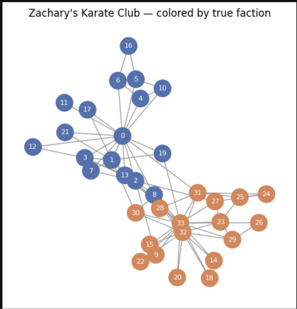
It looks like a spider web consisting of 34 nodes and 78 edges. Nodes are numbered from 1 to 34. They can have one of two colors (blue or orange). This indicates which class the node belongs to.

Next, there is the matter of information in a graph. You could imagine that these nodes could be colored in any way, and any node could also connect to anything else. If there is no pattern to learn, it means that even if you give me part of the graph, you cannot predict the remaining portion.

The above case is different, however: we can see two separate clusters. If we somehow learned how to group the blue and orange regions together, we could tell which nodes belong to which cluster. The problem then boils down to representation. So let us get started.

We can represent our graph as an adjacency matrix. Each row represents one node (let us call it A). Each column represents all the nodes that A is connected to (let us call it B). A value of 1 in row A, column B means that A → B. The graph above is undirected, meaning that a connection goes both ways: if A → B, then B → A as well. We can represent that by setting the B-th row and A-th column to 1.

import torch
# build graph 
# --- Adjacency matrix (no self-loops yet) ---
A = torch.zeros((N, N))
for i, j in edge_list:
    A[i, j] = 1.0
    A[j, i] = 1.0    # undirected graph -> symmetric adjacency

print(A)

# note: self loop is required because a node needs to be able to `see' its own features
# --- Add self-loops: N_i now includes i itself ---
A_hat = A + torch.eye(N)
# A_hat = A
print('a_hat', A_hat)

If we try to plot our graph, it looks pretty cool like the image below:

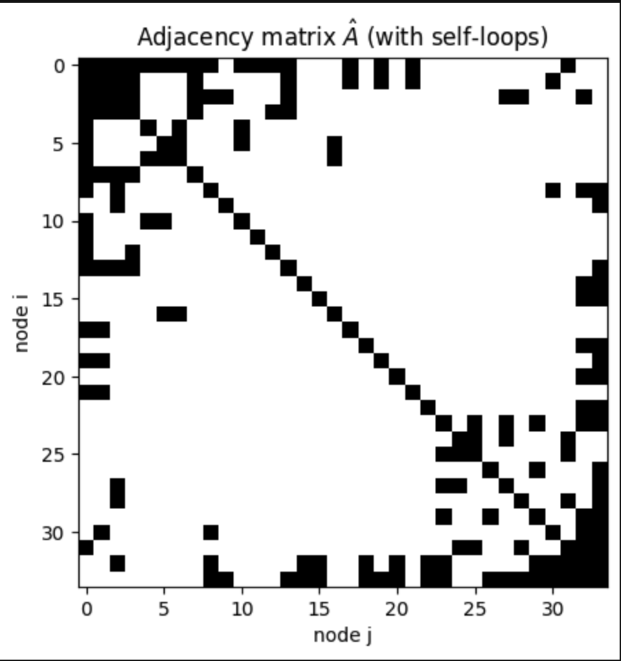
Note that the diagonal is all black. This means that particular value of the matrix is 1. (the way i plotted it, 1 means black). Similarly, a[i][j] = a[j][i]. This means that the graph is `symmetric’. You could imagine the above image as a sheet of origami paper. Next, put a ruler along the top left-> bottom right diagonal. Then ‘fold’ the paper along that ruler. The upper triangle and bottom triangle will overlap with one another. Please note that this representation only encodes ‘connectivity’ of a graph, i.e. how does a node i connect to node j. It contains NO information about what nodes i/j themselves represent. For eg, node i could be a fifa player, some user in a social network, or whatever.

The key point is that a graph has two components to its representation 1) connectivity (which above representation achieves) 2) what the nodes mean? We call this node-features. So, how can we represent the nodes of our graph.

Turns out the answer is pretty dumb. There are 34 nodes in our graph. For each node, we can create an array of 34 elements. The `index’ which corresponds to node id is kept as 1, and other nodes are kept as 0. People like to call it one hot encoding. As you can see, we are only setting 1 element of array as 1, and the rest 33 as 0. If there are billions of nodes, then for each node, there will be billions of columns. It will get messy really fast, but we won’t get into that right now. For now, we assume our graph is beautiful, and won’t expand beyond 34 nodes.

# --- Node features: identity matrix (one-hot per node) ---
X = torch.eye(N)
print("Feature matrix shape:", X.shape)
# node features are one-hot encoded

plt.figure(figsize=(5, 5))
plt.imshow(X.numpy(), cmap='Greys')
plt.title("Node features matrix ")
plt.xlabel("node j"); plt.ylabel("node i")
plt.show()

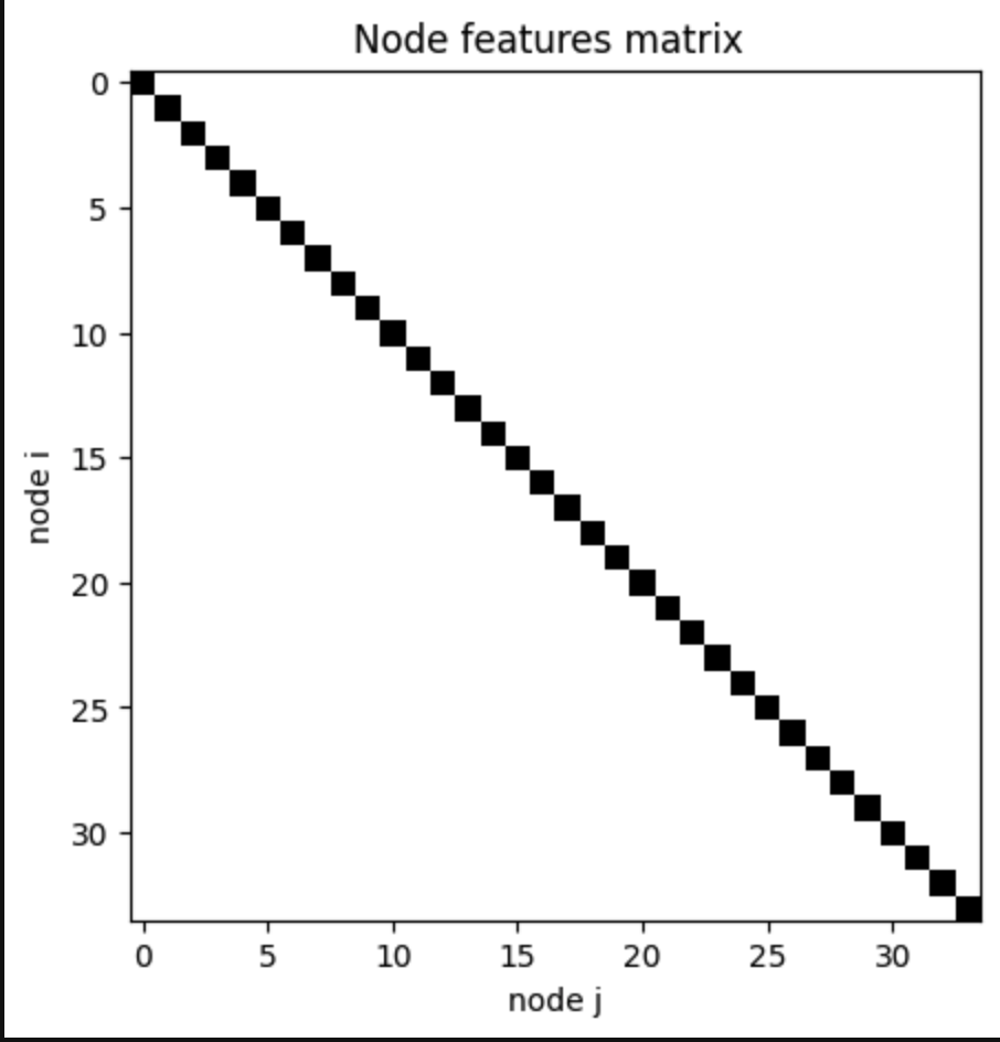
If you try to visualize it, it looks like this cute black diagonal on a white sheet of paper. Mathematically, this looks like a 34 by 34 matrix. So, now you can imagine that `each’ node comes with a 34 dim vector and there are 34 such nodes. Your figure starts to look something like this:

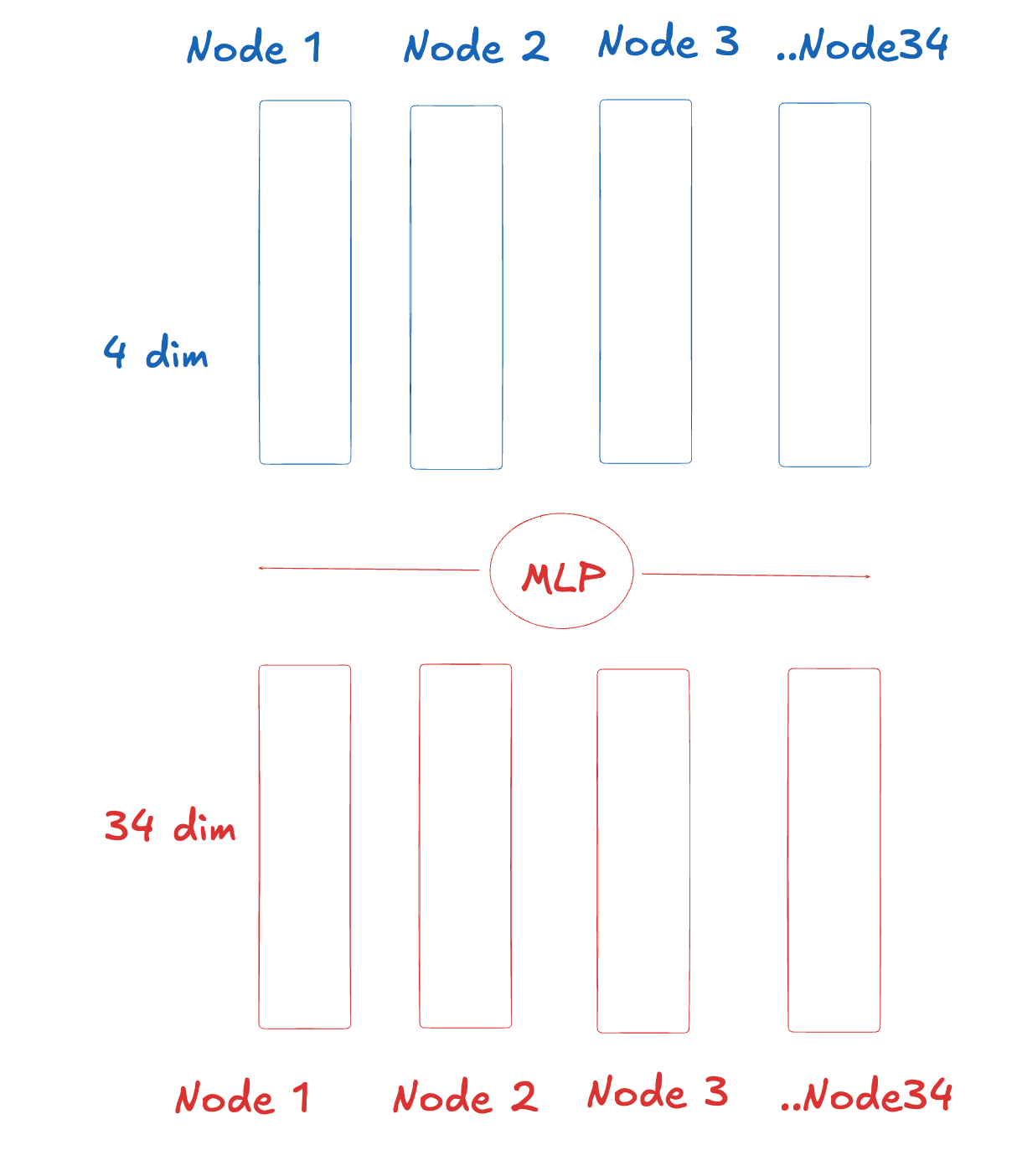
You can think of it like this… at the bottom level there are these red columns, length of each is 34 dimensional. There are 34 such columns (hence nodes). You can shoot each column into a MLP. The MLP transforms these columns into 4 dimensional columns. You will ask: `hey dude? why did your mlp transformer a 34 dimensional column into 4 dim’. The answer is compression: the ‘red columns’ are one-hot encoded, but 4 dim columns will have some non-zero value in each of the 4 slots. Since you reduced 34 dim to 4 dim, you gained a compression factor of 34/4 = 8.5!!.

Now, we can ‘throw’ away the MLP. It has done it’s job. It has already given us the blue columns representing the nodes. Recall that the graph contains a ‘connectivity structure’ also. We need to `somehow’ teach our neural net which node is connected to which. In other words, we need a mechanism which teaches a node i to ‘talk’ to it’s neighbors j.

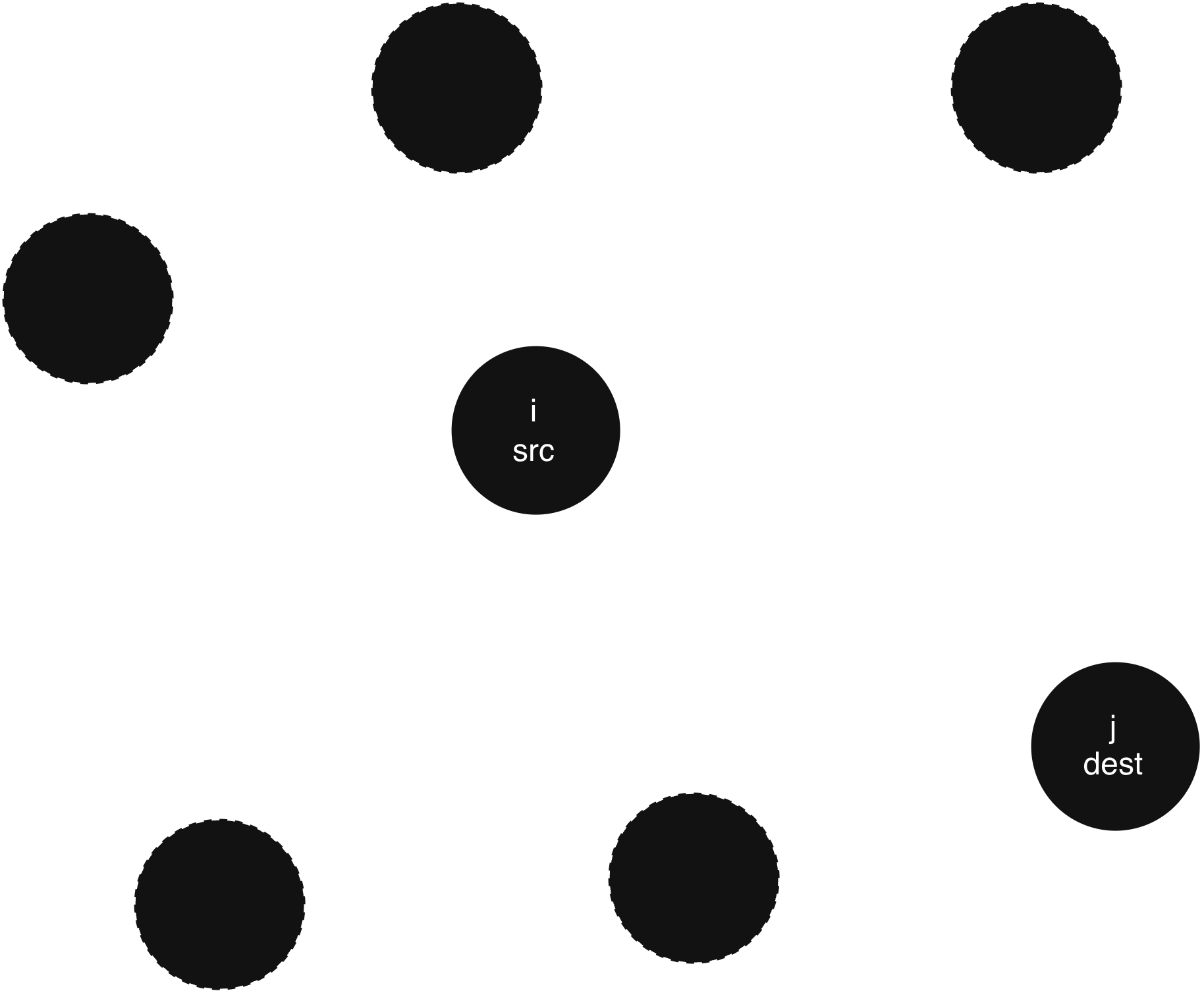
We can call the figure above as a `talking graph’. Here a node $i$ will talk to its neighbor $j$. The actual talking mechanism is best understood by the following figure.

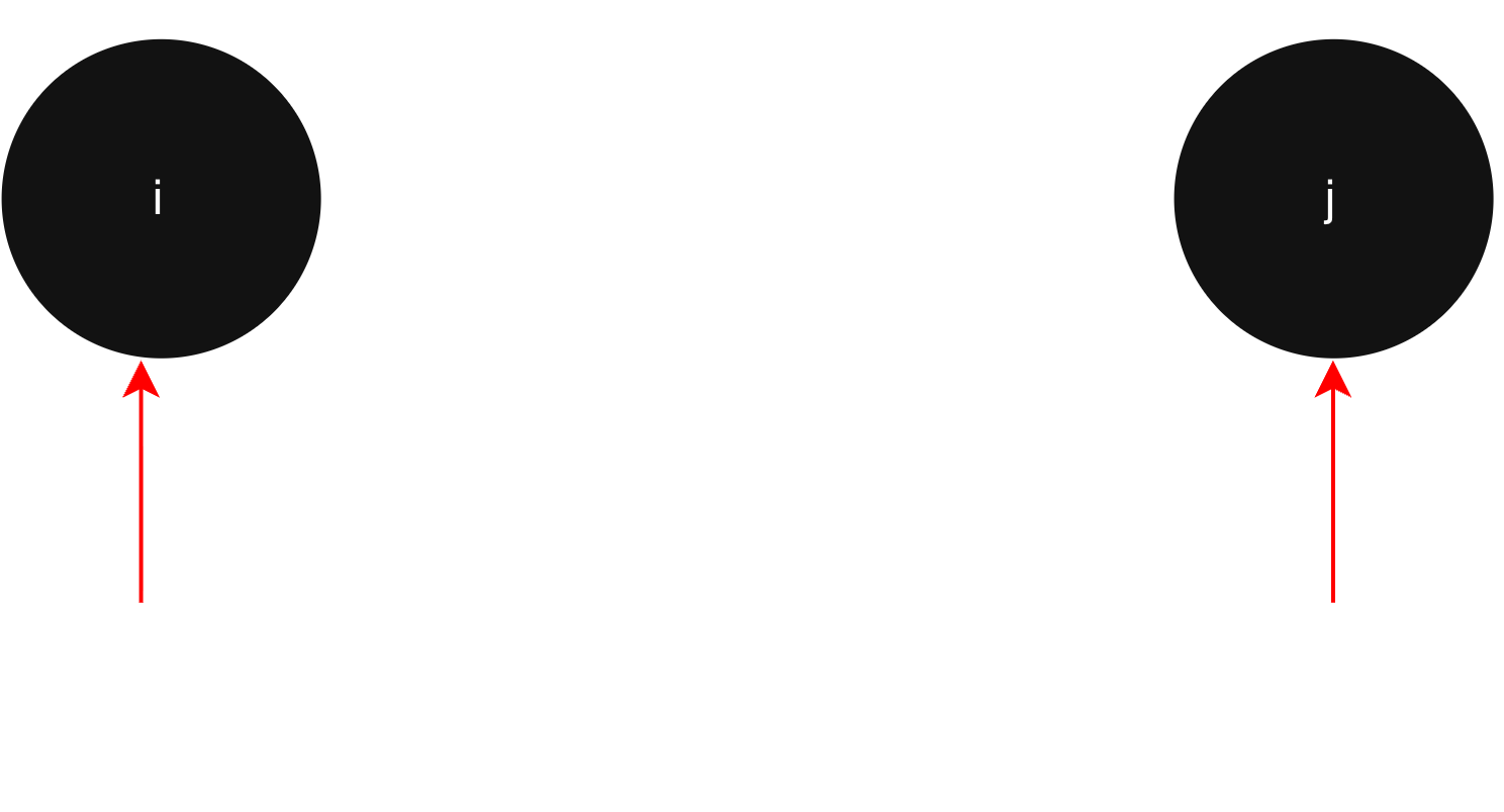
Instead of going into the math, let us imagine a conversation between a node i and node j. First our dude i is thinking what to ask j. Here’s what goes inside i’s head.

Node i: Geez, my input vector is node vector i. I am a little guy surrounded by all these j’s in my neighborhood. My vector i looks a little bit off. I must try to correct it. So, let me ask my neighbor j for advice.

At this point, our little node $i$ is deeply unhappy. So, what he emits a query to node j.

Node i: Dear j, this is my current state. Can you tell me if it’s good?

Now our node j is a very kind person. He listens to i. But he is all about vibes. He can never say no to anyone who asks for advice. So he does what he does best.

Node j: Sure i, here is what i know (key(j)). Use from it what you will. I have told you all i know man, but you must make a judgement of `what’ you take from me.

Our node i however a noob. He has no judgement. So he says:

Node i: `Woah, you are so kind. I will just add whatever you gave me to myself. We will vibe together’.

So, our dear node i then computes a relevance score by just adding his query with the key the kind j provided to him.

But here’s the kicker. Our dear i has many friends. He wants to vibe with all his neighbors j.

So a lot of j’s shared their vibes with i. Let’s call those vibes (relevance) as vibe1 vibe2 vibe3 .. and so on. Now, our dear i is confused. Here thinks:

Node i: OMG. I got so many vibes from all my friends. There are $N$ friends , and they sent me so many vibes. But, i have only one input node vector $i$. How do i take all these vibes, and `transform’ my node vector i. Well, one option is just to weigh them properly. Whichever friend j gave me more vibes, i will fluctuate my node vector i in that direction.

So our i calculates `relative weights’ of all the vibes. For eg, for his friend 1, he does $\frac{vibe_1}{vibe_1+vibe2+…vibe_N}$. And he multiplies his node $i$ vector by that amount. Then, he sums all these ‘relative vibes’ from all the neighbors together, and get’s the final node vector i.

And that dear friends, is how graph attention networks work. It is possible to compress all the story above in the following code:

a_src = torch.empty(F_out, 1)
torch.nn.init.xavier_uniform_(a_src, gain=1.414) # 1 value query emitted for simplicity

a_dst = torch.empty(F_out, 1)
torch.nn.init.xavier_uniform_(a_dst, gain=1.414)

# coupling

# compute src representation
p1 = Wh @ a_src # n by d_out

# compute dest representation
p2 = Wh @ a_dst # n by d_out

mixed_coupling = p1 + p2.T # additive coupling, multiplicative is done in `other paper`, not bengios work

e = F.leaky_relu(mixed_coupling, negative_slope=0.2)

mask = A_hat > 0
e_masked = e.masked_fill(~mask, float('-inf')) # please note the masked bit flip, that's important

# apply softmax
alpha = F.softmax(e_masked, dim=1) # along every row, so sum of every row should now become 1

h_prime = alpha @ Wh

Woah, it is a mess!! Let’s break it down. $a_{src}$ is how our node $i$ transforms its node vector $W_{h}$ into a query it shares with all the folks $j$ around it. Similarly, $a_{dest}$ is the keys the node $j$ advertises to all possible $i$. Here, note that the value of $p1$, and $p2$ are NOT changing depending whatever a pair of neighbors are. This means that if $i$ has to advertise something to a few neighbors $j$, it will always `advertise’ the same vector. And this makes sense right: i has his own vibes, and he does not care what other people say. So he shares same vibes with everyone, and if someone likes him, cool.. If not, well i does not care, he will just vibe himself alone.

The second variable is what is called mixed coupling, focus on the line mixed_coupling = p1 + p2.T. Neither $i$ cares about his neighbors, and neither does $j$. They just take their vibes together and `add’ them. Note that the vibes are not multiplied here.

Next, we consider the above code from the perspective of $i$. He gets a lot of vibes from a lot of $j’s$. So he converts them to probabilities using the softmax term. Finally, he multiplies all the probabilities with his own hidden vector $W_{h}$ to get the final output. And that ladies and gentlemen, is what we call graph attention mechanism in our messy business lol.

So, now you can imagine a set of node vectors go in. A set of node vectors go out. And this block is a single layer of the graph network. And you have multiple layers of these blocks one over another trained with backpropagation yo. Inside each layer, this kind of game that goes on between $<i,j>$ is called a `gossip’ or an agreement phase.

adjacency matrix supervision: The actual graphical structure is injected into the network by enforcing an adjacency matrix representation onto the attention matrix. Please look at the code below:

e = F.leaky_relu(mixed_coupling, negative_slope=0.2) 
mask = A_hat >0
e_masked = e.masked_fill(~mask, float('-inf'))

Basically, each layer of the neural net is computing these attention matrices $A$. We want to encode this graph structure as this attention matrix. What this means is that element e[i][j] will be `attended’ to if $i\rightarrow j$. At each step, we shall ‘enforce’ this graphical structure inside the net. This is done by multiplying the attention mask $e$ by a ground truth mask $\hat{A}$.

Put simply, there are a lot of such graph layers. We feed them node embeddings. And we `force’ the structure of connectivity by supplying it $A_{hat}$ externally. In this way, the neural net can encode graph structure in itself.

Now that our little neural net is all wired up, it is time to train it on a toy task. So, let us first recall the graph earlier in this post.

We begin with a task called semi-supervised node classification. I know it’s a mouthful, so let’s dumb it down.

The graph contains 34 nodes, 17 blue, 17 orange. We will teach the network only 2 nodes (one node from blue cluster, and one node from orange cluster). We will not give it labels for other 34-2 = 32 nodes. It’s job is to infer the labels of remaining 32 nodes. If it does a good job, it will correctly predict other 32.

The kind of coupling we have built earlier in this post, should be enough to allow the nodes to propogate information among each other, and that should in turn allow our network to predict labels of other 32 nodes.

A snippet of training code looks like this:

train_idx = torch.tensor([0, 33])
logits, attn1, attn2 = model(X, A_hat)
loss = F.cross_entropy(logits[train_idx], labels[train_idx])

we are only choosing nodes 0, 33 to supervise, remaining nodes are masked. Train graph looks like this:

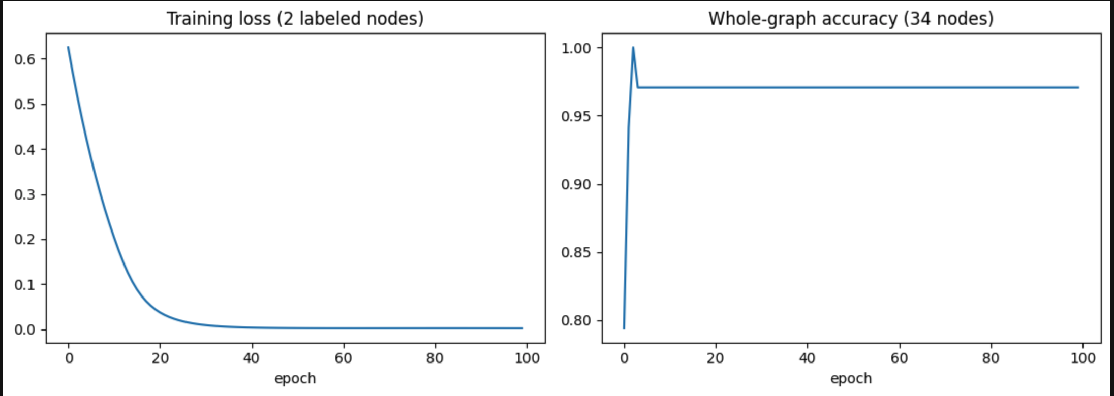
As we see, the accuracy peaks in mere 10 iterations, which means that our messaging passing in the internal layers of graph network are working. Once it’s done training, we can look at the intermediate representations of each node embedding, perform t-sne/pca reduction on it, and visualize the cluster, as shown below:

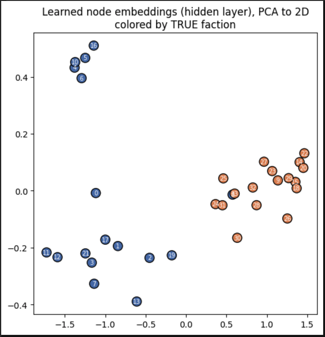
We can see the net was able to cluster these two together. At one node (Around node 33), there is one blue node, which means that it is making mistake in predicting the node embedding for that blue node. But otherwise it is doing fine.

Scaling up

There are a few things that stand out. The network is able to learn on just one graph. It only needs two nodes to learn, and the internal message-passing mechanism takes care of the rest. It is then possible to use the same network for different tasks:

Suppose a given problem is defined by many graphs, such as proteins and their structures in protein folding. The problem here is to learn the protein structure. We can assume that we are given many proteins and their structures. Then we can train the network at scale. Finally, given an unknown protein from the same problem, we can infer its structure. We can also predict which class each node belongs to, or predict the angle between nodes in 3D. We can examine all the angles and measure torsion or overall mechanical stress on a protein.
The limiting factor here is that the network trained in this way will work for only one problem (that of protein folding). The underlying assumption is that there is a set of weights that can encode the universal graphical structure of all proteins. As long as that remains true, the network will learn.
You could also use it for recommendation systems, road networks, social graphs, and whatever else you can think of. A lot of computational problems can be modelled as graphs.

Limitations

There are several limitations in this model:

There is all this machinery of parallel attention heads, and shrinking the embedding dimensions into bins. It really messes up with my mojo.
Node $i$ is sharing the same amount of vibe with all the neighbors $j$ in the first phase of the agreement process. This might not make sense. If you are a timid person and you talk to a muscular person, you may feel intimidated and become afraid. If you talk to a friend, you may feel comfortable. So the way you speak depends on who you are talking to. The model above does not capture that nuance.
The coupling between $i$ and $j$ is additive. It needs to be multiplied, but that issue was fixed later in variants such as Graphformer.
The mechanism has to input node vectors into the transformer/graph layer. The graph structure needs to be injected from the outside to each layer. This means that the learning signal has been decoupled. Information has to be injected into the neural net from two separate places, which makes it look ugly. Perhaps a better way exists.
It requires us to know the nodes beforehand. Suppose our problem is as follows: we are given an image and want to build a graphical structure from it. That means the input is an image, not the nodes. So how does node formation happen inside the neural network?
Encoding multiple graphs: Suppose there are multiple possible graphs for the same input. How does a neural network store all of them together? There are multiple possible answers, and right now there is only one $\hat{A}$ matrix that can be used to supervise the graph. This is a very interesting problem, and we should keep it in mind. There are some exciting ways to solve it, so I will discuss them in another post.
Flattening graphs: The original work in semantic parsing chose to model graphs as a serialized form. The basic idea was that graphs could be flattened (using some depth-first search and noting a node’s parents in the suffix of the sequence) and then used to train a sequence-to-sequence model such as a transformer.

There are two conflicting arguments here: (i) we care only about breaking a sentence into parse trees, and transformers do that quite well, so part-whole parse trees are solved; and (ii) the second argument is that we are still treating a graph as a sequence. Perhaps that is wrong. Or maybe we are wrong.

Now we have finally reached the end of the post. We have done a lot of hard work together in trying to build our intuitions. So now we deserve to have some fun. We will recall Shin-chan’s bori bori dance from our childhood.

we love shin-chan. Maybe you should too.

until we meet next,
love,
rajat