P.S. Apologies for the wrong spelling. Force of habit.

Recently, I had the privilege of attending a talk by Takeru Miyato, on his ICLR 2025 oral paper titled `Artificial Karamuto Oscillatory Neurons’. The idea seems pretty interesting, and authors have done a great job explaining their paper in great detail here.

I cannot do justice do their amazing work, and really urge the reader to look at their original work (and followups) for a detailed understanding. Here, I will merely attempt to distill some of their key points, in the hopes of building a better understanding, for the kind reader. First, we cover what is known in neuroscience has the binding problem.

Binding Problem

Around 60 years ago, people got interested in how we can look at an image, and automatically cluster different objects together. For eg, if the image contains a cup, glass, then we can automatically group them into corresponding regions.

Suppose you are given a blue cup, and a red cup. Somehow, the brain is able to combine the representation of “blue” with “cup”, and “red” with “cup”, to yield two different representations for blue cup/red cup respectively. There are two plausible arguments here. (i) brain has learnt separate representation for blue cup/red cup. Given such an input, it just “selects” the correct representation out of a dictionary of objects. (ii) brain `dynamically’ combined blue and cup together to form blue-cup on the fly.

A criticism of (i) is that there are infinite objects, and their combinations available, which means we don’t learn a massive superset. Rather it seems that we rely on (ii): learn only a few abstract concepts like colors, objects, and combine them whenever needed. This second problem is known as the binding problem.

The key issue is : 1) how does this combination actually happen? 2) given an image containing both blue-cup, red-cup, how do we `simultaneously’ maintain two-different representations at the same time in our heads?

The hope is that by figuring out how these different attributes combine during inference, we can get better generalization on objects we have never seen during training. Classical AI will just train model on separate samples of blue cup, red-cup, and hope it figures it out. But, that didn’t work quite well.

Static Learning: Mccullough Pitts Neuron

For almost 50 years now, the fundamental unit of AI had been Mccullough Pitts Neuron (MCP): it has served as a simplistic model of biological neuron: the core idea being that inputs are multiplied by some weights, summed up, and squeezed through a non-linear activation. Thus, it is a kind of static neuron: once the input comes in, there is no delay, and the output is a mere consequence of a few multiplications and additions.

One bitter lesson was the realization that albeit simple, this neuron serves us quite well: it scales easily, is massively parallelizable, and forms the backbone of the majority of language models we see today (LLMs). The efforts spent to simulate `more biological neurons’, for eg, via spike trains eventually underperform, or perform similar to MCP.

Towards Dynamical Systems: Karamuto Neurons

There appears to be another kind learning principle possible, the one called `synchronization’. In nature, we often observe flocks of birds, or swarms of ants, which always seem to agree on some patterns w.r.t each other. For eg, birds always travel in a triangular formation. An ant follows the ant before it, by smelling the pheromones the latter releases. If there are more ants on a single path, they release more chemicals, thus strengthening the ant’s probability to follow that particular path, rather than other paths where the chemical signal is weak. Similarly, fireflies twinkle in a rhythm.

Fundamentally, these patterns in nature seem to emerge when, we build a system with massively interconnected components, and just allow them to interact with one other. As the time proceeds, this system eventually settles in a state of minimum energy. Think for eg, an isolated container of heated gas, kept at room temperature. Eventually, it will cool, reach thermal equilibrium. Even at constant temperature, however it’s internal molecules keep changing positions (brownian motion), thereby exhibiting multiple states. This kind of system is called a `dynamical system’.

This raises a question: Can we build this fundamental principle of synchronization in our existing neural nets? Will it help us arrive at certain new kinds of properties?

Fortunately, such form of dynamical properties can be accomadated in neurons, using a model called `Karamuto Neuron’. Next, we discuss this idea further.

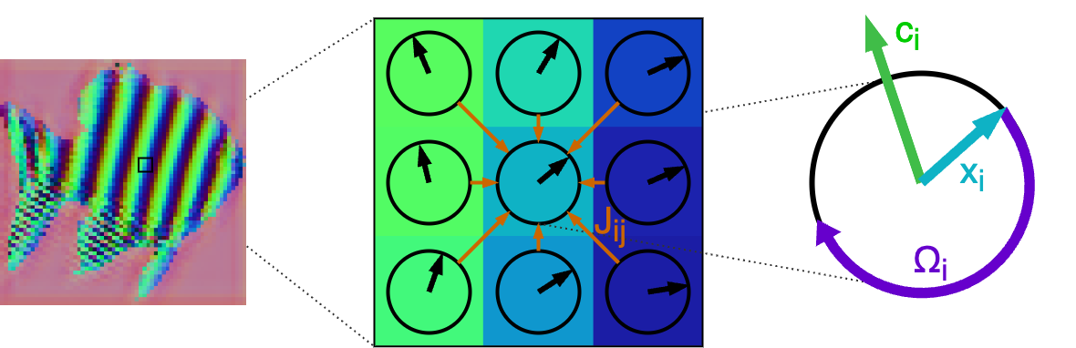
At its core, we can imagine that our neural network takes an image as input (in this case the fish image shown above). Each pixel in the image can be thought of containing a vector of $d$ dimensions. So, for $H \times W$ image, we have $H \times W \times d$ vector. At `each pixel location’, each vector has a phase, and angle. You can think of these vectors like oscillators, little tiny arrows which rotate at their locations in the image, and are trying to orient themselves in the representational space, to perform make some sort of sense of the input data.

Next, there is this matter of coupling: how are nearby neurons wired with each other. Consider a vector $i$ in the center of the image. It will interact with neighbouring vector $j$ through a weight $J_{ij}$. Please note that this connection is non-symmetric, i.e. the weight $J_{ij} \neq J_{ji}$. Next, one can define an energy expression, which is subsequently minimized over several learning iterations. Before discussing math, it may be helpful to look at it intuitively.

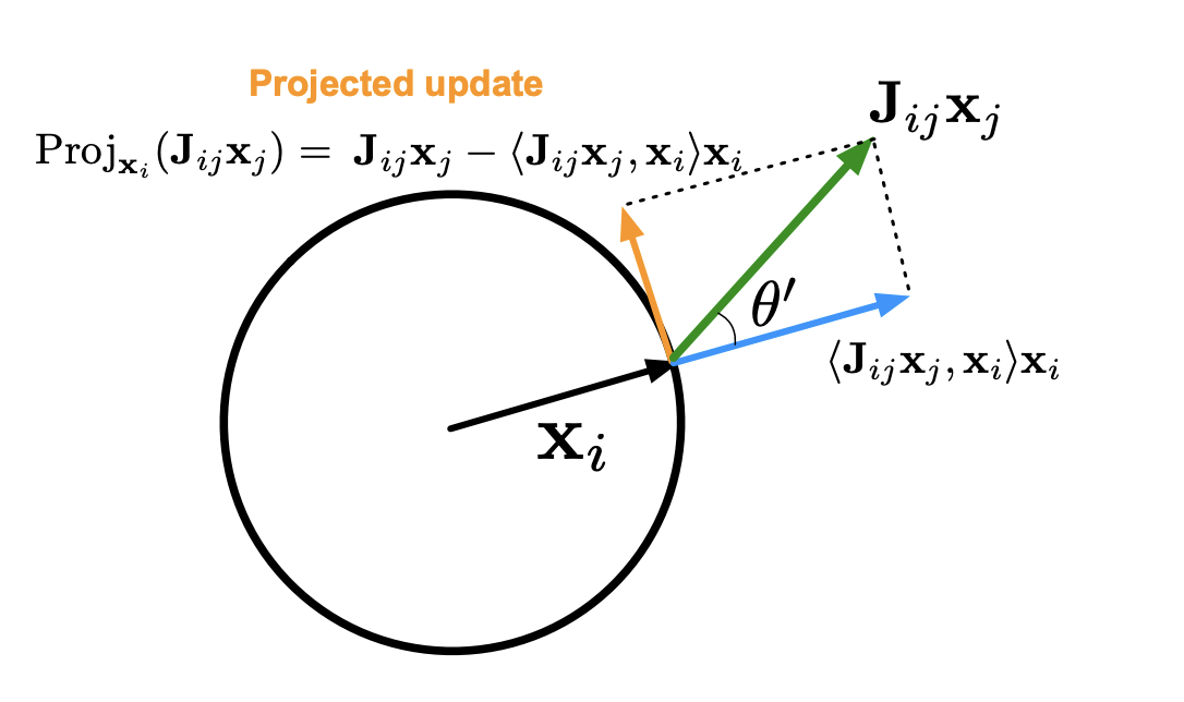
Please consider, as before, the coupling between vector $x_i$, and a neighbouring vector $x_j$. When we multiply $J_{ij}$ by $x_j$, we can compute how much relevant it is to $x_i$. Geometrically, this can be denoted by two arrows lying on a hypersphere. First there is an arrow $x_i$, in a unit radius (after normalization). Next, there is an arrow of $J_{ij}x_{j}$, at some angle $\theta’$ with respect $x_i$. Please note that this is not of unit length, but some random magnitude. Also the product $J_{ij}x_{j}$ is a vector, which means $J_{ij}$ is a vector of weights, and not a singular value.

Once such a view is imprinted in our minds, we want to define an energy function. The constraint we want to promote is one of `synchronization’, i.e. these two vectors should synchronize, and converge to same angle. Intuitively, we want $theta’$ to become 0. An alternative way is to consider the tangential projection $J_{ij}x_{j} - <J_{ij}x_{j}, x_{i}>$. By minimizing this length, we can ensure only the component of $x_j$ in direction of $x_i$ remains. If the length becomes 0, it means that these vectors are in perfect synchronization. The energy function of this system can be defined as:

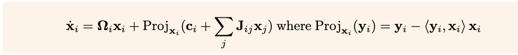
It is easy to imagine this equation as a differential equation. Basically, we can imagine that the vector $x_{i}$ is gradually changed by all the vectors $x_{j}$ connected to it. We can sum up the total tangential length error of each pair (i,j), and try to minimize it. The left term containing $\Omega_{i}x_{i}$ means that the vector $x_{i}$ is rotated by certain amount given by learnable matrix $sigma_{i}$. You add the left term and right term together and voila: you get $d(x_{i})$.

For several iterations, the vector $x_{i}$ is refined by different $d(x_{i})$, and finally gives the final value of $(x_{i})$. This is what the authors mean by a Karamuto Step. It is shown in the figure below:

At each layer, the network performs $T$ such iterations. Given a particular $x_{i}$ and a given $d(x_{i})$ at each time step , the karamuto step was defined as: $x_{i} = \pi (x_{i} + d(x_{i}))$, where $\pi$ was a normalization operator, pulling $x_{i}$ back onto hypersphere. And the main point is that if you are making the above step, you are actually minimizing the free energy of the system. If you continue taking these steps, eventually, the neurons in the neural-net will start to synchronize. What we mean by synchronization is the figure below:

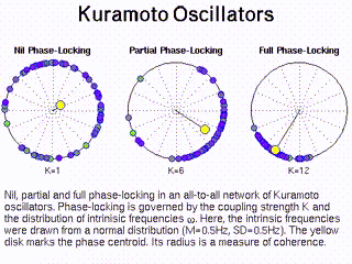
On the left part, all oscillators are random and they have no order to them. In the rightmost figure, we achieve a phase lock, where different oscillators have bound to one another. You can see just a single blob of purple, so it means that, right now, the oscillators think that they are part of the same object.

Next, we must convince ourselves of another subtle fact. Let’s look back at the equation again.

This equation is a function of $x_{i}$, $x_{j}$, and learnable weights $J_{ij}$. Even if the weights are not changed, (there is no learning happening), the vector $x_{i}$ will still keep changing. And synchronization will still happen. This means that by just performing several such karamuto steps, the neurons of a network can synchronize. Hence this step does not need learning algorithm.

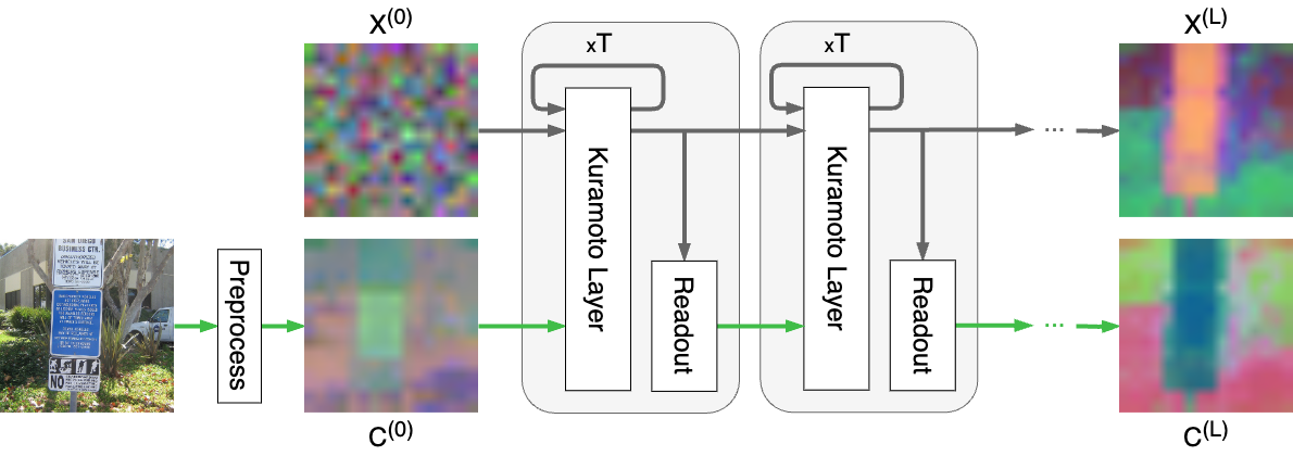
This internal karamuto dimension denoted as $T$ in the figure, then becomes an inner TTT loop. In the outer loop, the actual weights $j$ are changed, with task specific backpropagation loss.

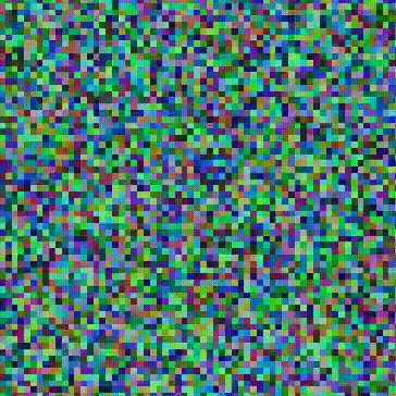
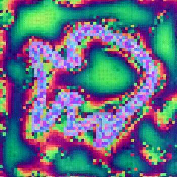
So if you take a single image, and run karamuto steps on it , you will eventually end up with certain wavy patterns of the kind found in the brain, also known as travelling waves. For eg, consider the fish given below:

This is a consequence of running many karamuto steps on it. Note that this procedure didnt require any learning, but only the existence of weights $J$ as a bridge to make different locations $i, j$ communicate with each other. Looking at the figure above deeply, you will notice the background is pink. This means that oscillators in that region are not changing, which means that the input image explicitly marks those region as 0 (and indeed paper does, godammn,:-), ).

Now we must we wary, because if we remove this (a.k.a. masking the background), and allow the entire image to evolve, it will lead to chaotic patterns like these:

Interestingly, these patterns are what John Conway’s observed in his game of life. The key difference in that it was for 2D, and this is for RGB image.

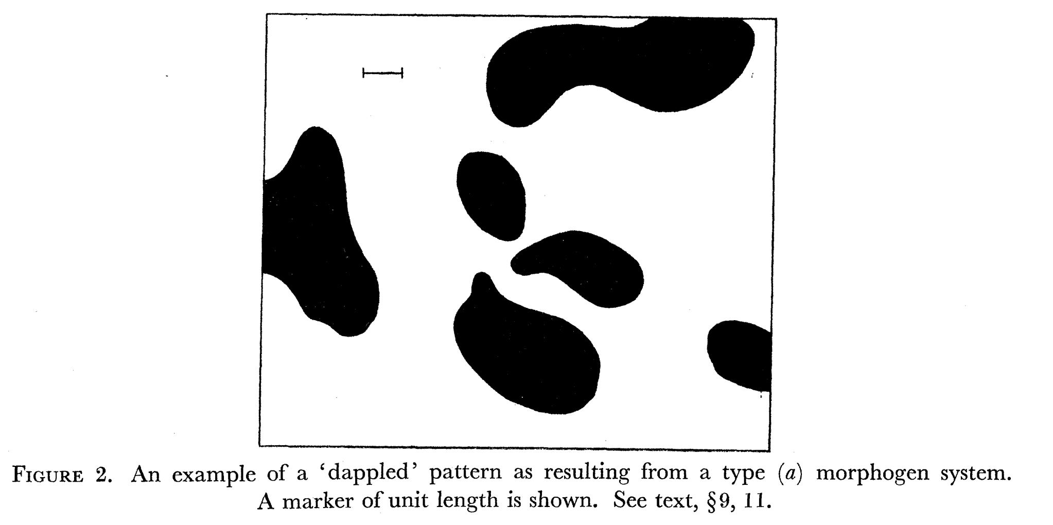
Above figure is from a paper titled `Chemical Basis of Morphogenesis’ where scientists as far back as 1930’s discovered such interesting patterns forming.

We must now reorient ourselves and distinguish between a chaotic and periodic pattern. The above pattern (of the fish image) is chaotic, and much different from the wavy pattern earlier. It feels as though this particular chaotic dynamic will not lead to good representations. However, this pattern as well as the pattern above are both periodic: they repeat after a period of karamuto steps.

Stacking More Layers

An important question thus becomes: what happens when we stack layers containing such karamuto neurons. Indeed, the authors experiment with this:

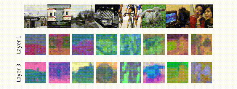
We can run each layer for $T$ karamuto steps, collect latent features, and perform 3D t-SNE reduction on all of them. And play those rgb frames for each timestep as a video. We can observe that lower layers change rapidly (thus operating at higher frequencies, explicitly capturing finer part-level details), and gradually grouped into stable clusters which don’t change (thus lower frequencies of oscillation).

We must yet convince ourselves again: At higher layers (layer 2), look at the bottom left square. You will see the the sky in bottom left becomes pink. This means that the representations in the pixels corresponding to sky are not constant, but merely oscillating. Thus, the different regions are “binded” together, but are rotating in a higher dimensional space, but kinda stuck together (like a phase-lock). You can also think of it as a spaceship, which has all it’s parts glued together, and travelling in space.

Solving Sudokus

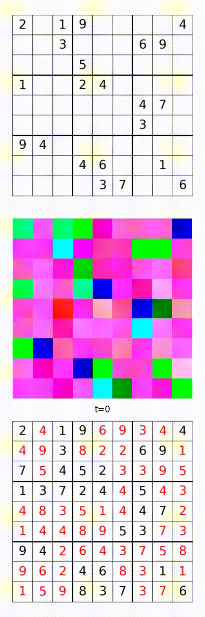
Karamuto neurons may be used to solve sudoku. Basically, it is a 9 by 9 square, containing 9 smaller boxes. We wanna fill it with digits, such that each box, each row, and each column contains 1-9 numbers, and there is no conflict. Indeed, there are infinite sudokus possible.

The kind of problems we are interested in involve the grids which possess a unique solution. Let us imagine there is a sudoku with only one square filled. There are many solutions to it. Therefore, a network cannot learn anything, unless we allow it to make multiple plausible predictions. Hence, for simplicity, we are interested only in one-to-one solutions.

Solving a sudoku is hard if it contains only a few filled digits, and you have to fill a lot more. So, it is possible to divide a sudoku into two parts, iid, (easier grids), and ood (harder grids). A network can train on iid, and test on ood, to evaluate generalization ability.

There are two notable properties of interest 1) authors show it is possible to solve iid sudokus with 0 standard deviation: this means that the network converges to a fixed solution, that perfectly solves it. Now, let us truly understand what 0 std means.

A neural net running in feed-forward mode, will always give fixed answers, (unless it involves sampling, which if kept fixed, will still give same answer). A machine can keep running until it reaches one of the solution and continously oscillates between different solutions, all of which are correct. Alternatively, a machine can reach a perfect solution, and just stop, much like the wheels in turing’s enigma machine. A machine if not sure, or not having 0 loss, will continously keep operating. Given a problem of similar hardness, (iid train, iid test, are both iid problems), the network can still stop.

The issue however, is in ood setup. This standard deviation is not 0 there, and the network still does not generalize that well. So, there may be a some work which can be done there.

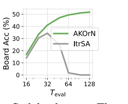
The second property of karamuto neurons is the additional latent dimension a.k.a karamuto steps. Even without an external label, the network can in principle be run till infinity. The hope is that the representation gets better over time, leading to better downstream performance.

In the figure above, authors show that if you run a transformer (a self-attention layer with output fed back into it) for several time steps, the representation degrades. Karamuto neurons, however remain stable.

Now, we must be wary. There are papers like Deep Equillibrium Models (DEQ), whose core argument is that a network if ran till infinity, will reach a representation which does not change continously. The issue is that, it takes too long to converge, and in practice, i believe it never does reach a stable representation. Also, the performance of the network `need not be best’ once this singular point is achieved. No one has yet shown that there is correlation between singular point, or the best performance. Indeed, this phenomenon is called deep-thinking, where best performance peaks, and then drops. The singular point lies well beyond the iteration where the peak-performance happens.

Object centric Learning

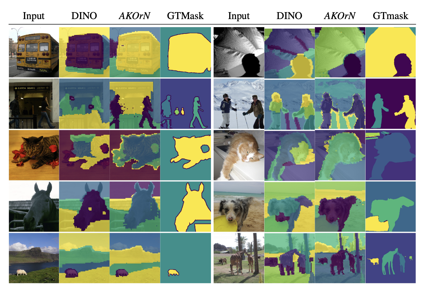
Indeed, it is possible to stack karamuto layers (in attention- connectivity), and train it on imagenet. Loss can be simple classification loss, with internal karamuto dimensions.

The key argument here is that such network can learn better object centric features than say (DINO). For eg, in the figure above, we can see that the object masks indeed look pretty cool. If you take DINO backbone, and refine those features by using karamuto layers, it gets even better, showing that this kind of learning can even benefit existing models. You can imagine inserting karamuto adapter-layers in between models, tuning only them.

Obvious questions

Indeed, several questions are possible 1) how well does it do on language task, scaling up 2) how robust it is to adversarial attacks 3) does it scale to real world 4) how does it do given realistic images containing many objects 5) how can this be extended to generation (Eg, diffusion), or reasoning.

Albeit important, i tend to view these questions as superficial. Reason being, you could ask these questions of any paper. None of these questions is explicitly questioning the `karamuto’ model itself.

As researchers, our job is to demonstrate viability: scaling up is indeed important, but that should not become the sole cause of our motivations, and indeed their are better people who specialize in this . One may argue that scaling, and fundamental research can go hand in hand: i don’t believe so.

This raises the questions: Are there any better questions we could ask ourselves? Indeed, i can only try to merely make a humble attempt. If you feel it may be of any help, please check our follow up post here.

Till we meet next,
love,
rajat