On energy based models

Course notes of stefano ermons CS230 lectures 11/12/13 at stanford.

The sun illumines the world, but the light is one. Similarly, the energy of the Supreme illuminates the whole world, and yet the energy remains one. (the sum of probabilities in energy based models also remains one :-))

If you are like me, you don’t understand how the diffusion models work. In fact, you tried reading it, but it didnt just make sense. The math just seems crazy, and it just seems like you have to memorize it to ace those interviews lol. Adding noise, denoising seems cool, but how the heck did they come up with it? Surely, the brain does not use such a process to “dream”/ “generate” new samples.

Recently, i had the privilege to audit stanford CS230. It is taught by Dr. Stefano Ermon, who also happened to be coauthor of several diffusion papers. So, without further ado, let us get in the trenches and learn directly from him. Here we are going to talk about Energy Based Models, namely lectures $11, 12,13$.

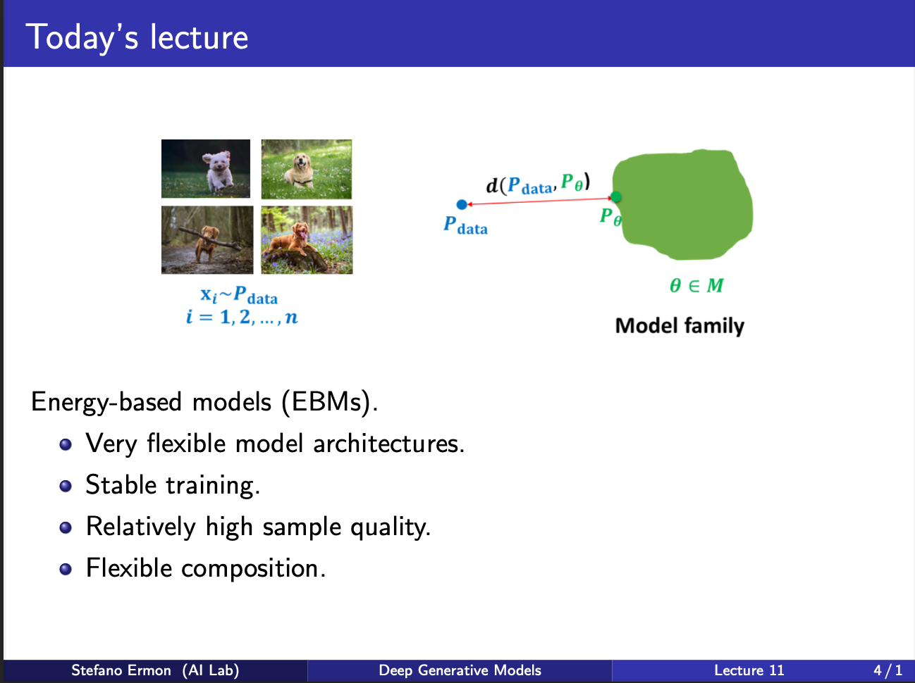
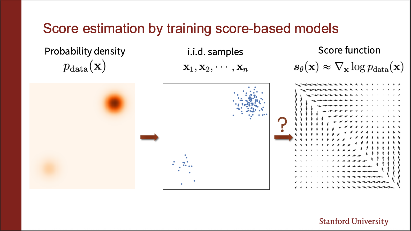
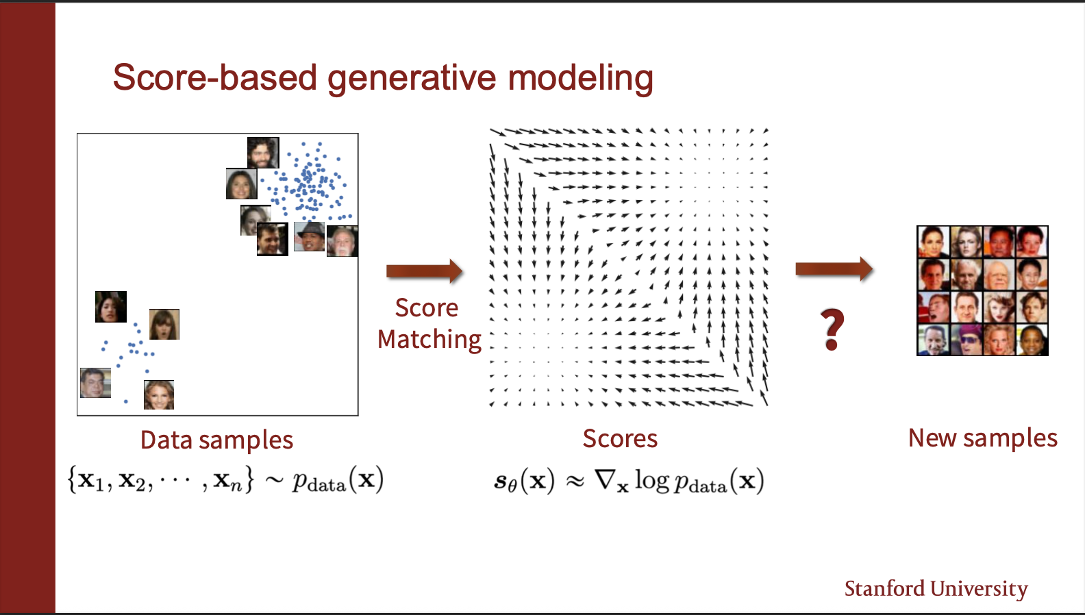
The core purpose of energy models is that they are very flexible. Consider that your input data comes from a ground truth distribution named as $p_{data}$. The aim of the model to learn a model $p_{\theta}$, which wants to approximate this $p_{data}$. So during learning, we will be given several iid samples $x_1, x_2, …..x_n$. We want to “fit” $p_{\theta}$ on it, and form a generative model. So, if we sample images from it, we should get new images never seen during training.

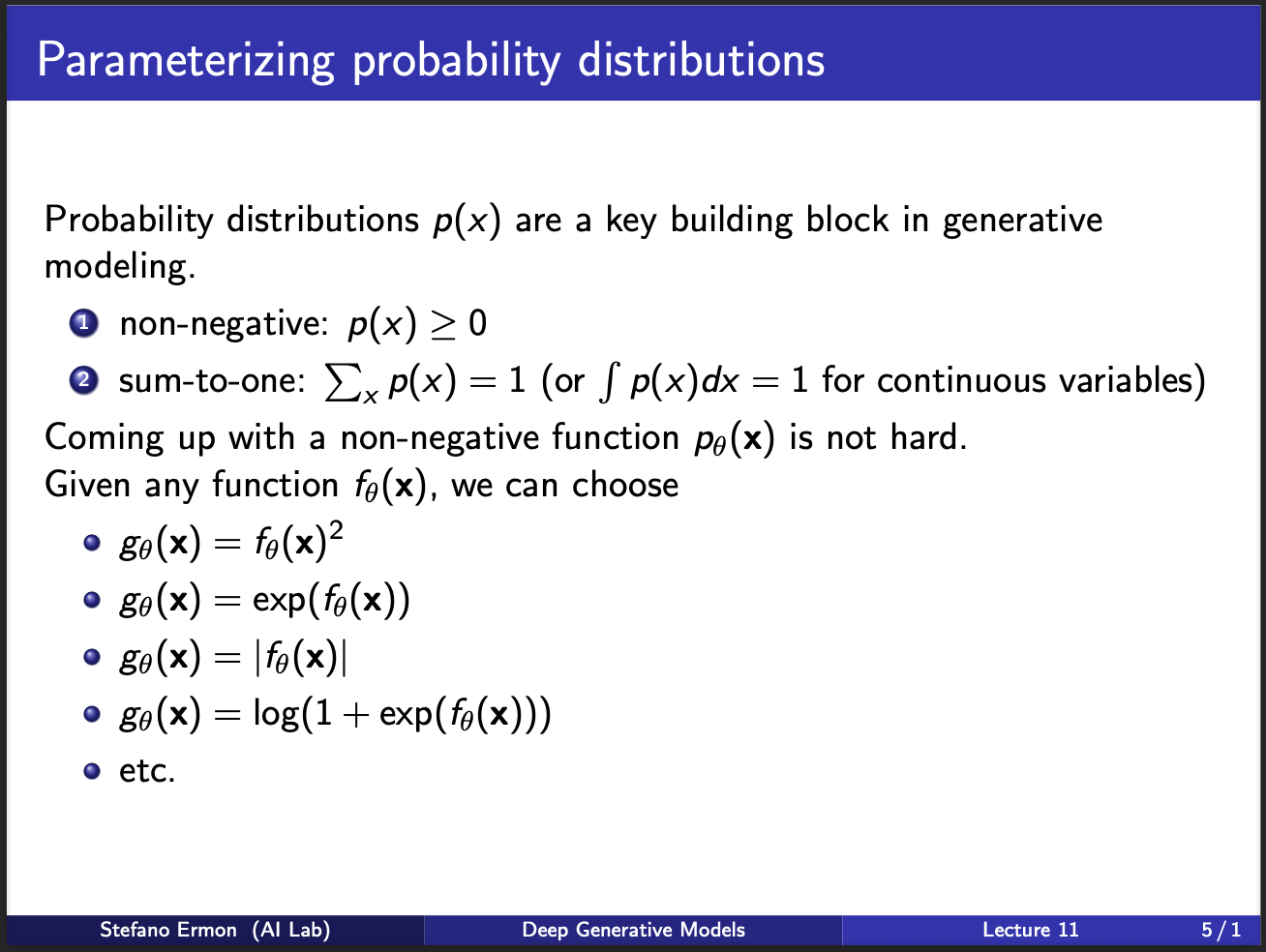
What are the properties that we want our model $p_{\theta}$ to satisfy. For now, let us call $p_{\theta}=p(x)$. For a given image $x$, the probability should be greater than $0$. Let us assume there are one million input samples, our model $p_{\theta}$ will spit out a million probabilities. The sum of these probabilities should be $1$. The next question becomes: How to choose the model $p_{\theta}$. In practice, several kinds of models are possible. As you can see in the slides, the output of $p_{\theta}$ is passed through an activation function $g_{\theta}$. So, there are several ways to choose this activation function $g_{theta}$. For eg, it can be a quadratic function, exponential function, mod operator, or a log sigmoid. Anything will work in practice.

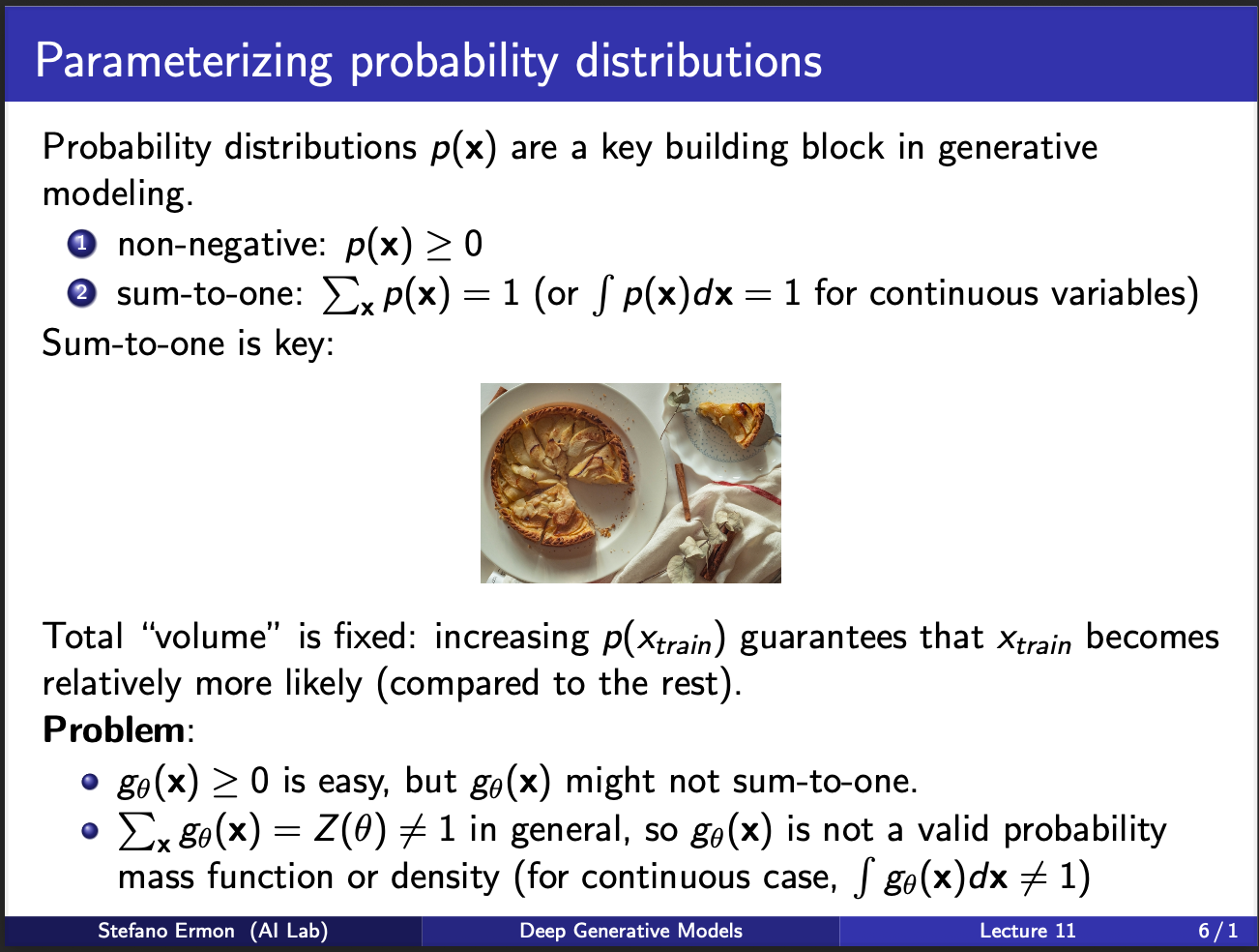
In the figure above, you see a pie. Intuitively, that pie represents a volume. Each slice of the pie represents the probability of occurence of a particular input sample. In case of million of samples, our pie consists of infinitesmal small pieces, the sum of which should be equal to entire pie. So let us say, that we pass a particular sample through the network, and get a value of 2. To calculate the probability of that sample occuring, we need to know the size of the total pie. This appears problematic due to two reasons: 1) you will need to feed-forward all plausible input samples to get their values (and hence the volume of the pie). This is not possible in practice, since we don’t know all the plausible images in the world. This means, it is not possible to get the total size of the pie which is denoted by $z(\theta)$ here.

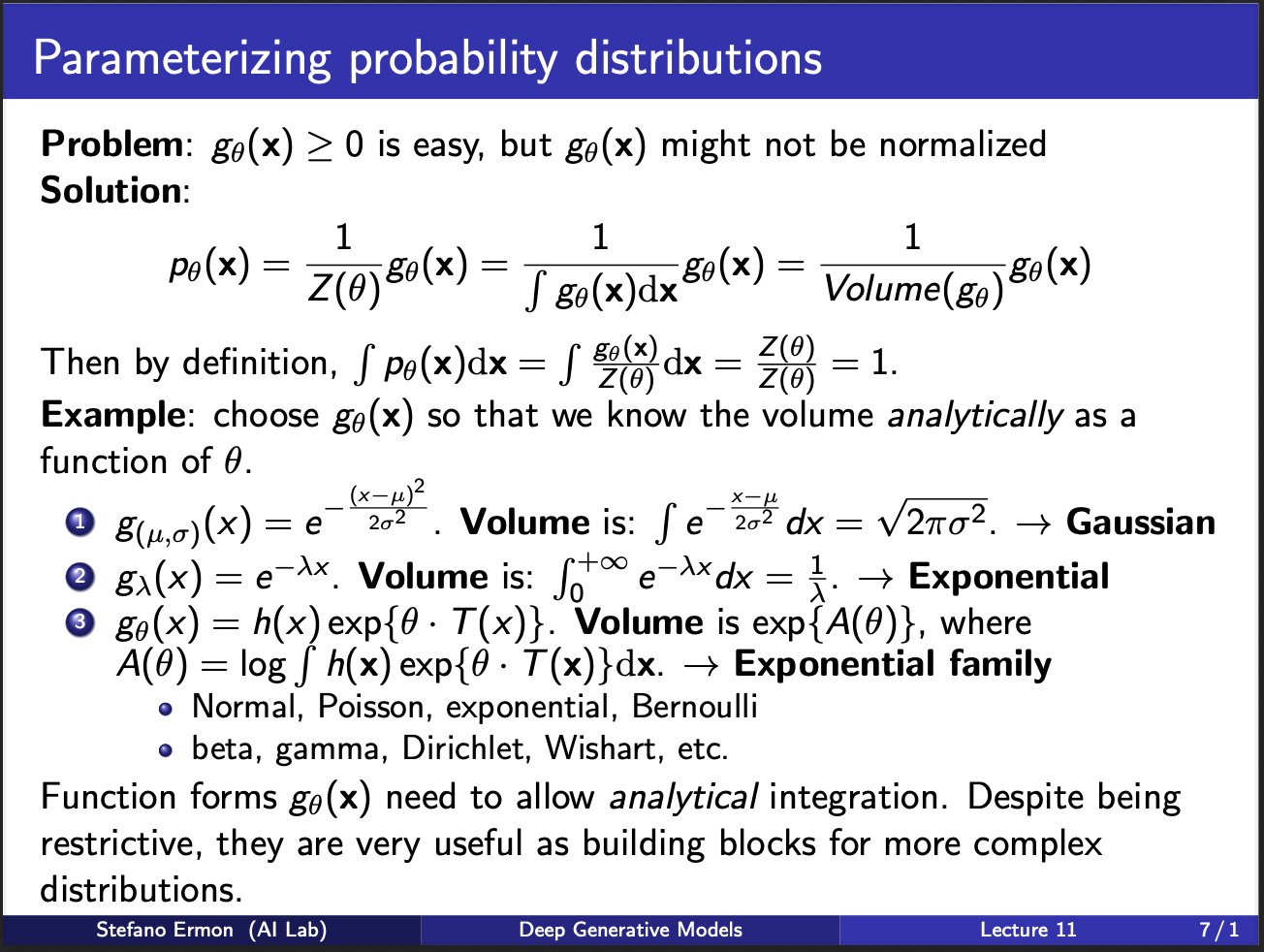
The way around this huddle is to assume that the “output” of a neural network, follows a preknown probability distribution. So, for sanity, let us assume that our output is defined by $g_(\mu, \sigma) = e^{\frac{(x-\mu)^2}{2\sigma^2}}$. This is equation for a gaussian distribution. Now, we `analytically’ can integrate this function over a plausible values of $x$, and get $\sqrt({2\pi\sigma^2})$. Note that this calculation required us to make an assumption: i.e. the outputs of our neural network follow a normal distribution. On surface, it seems weird to make such an assumption. On the other hand, the law of large numbers says that if we take a lot of samples, they tend to follow a normal distribution. So, it means that our assumption might not be wrong.

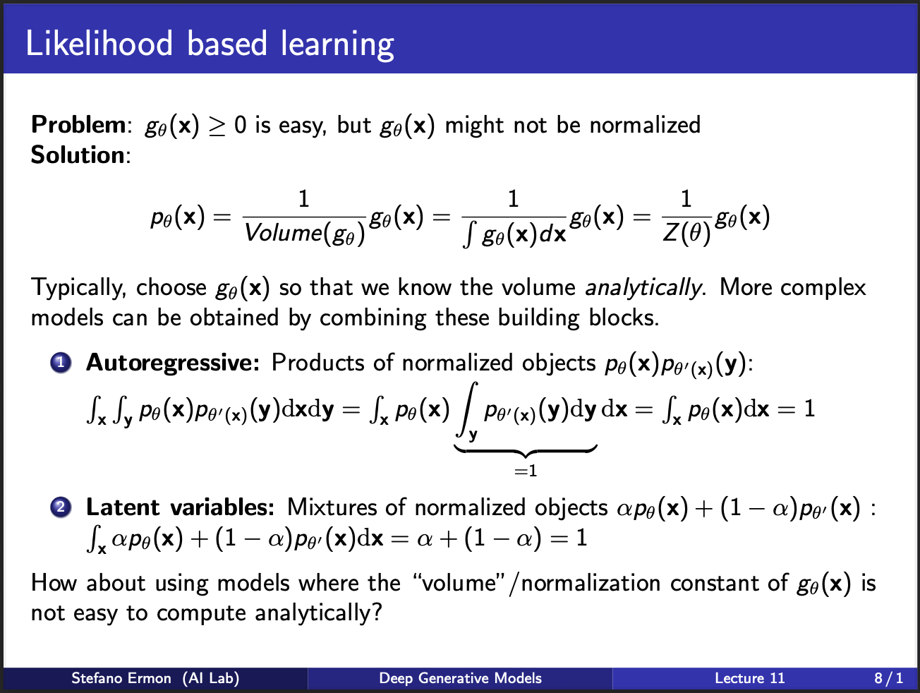
Assuming that we can integrate our $g_{\theta}(x)$ analytically, it becomes easy to calculate the likelihood $p(\theta_{x})$ by simply dividing $g_{\theta}(x)$ by its total volume $z(\theta)$. This $z(\theta)$ is also known as a partition function. Now, one can imagine that there are several such “neural nets” modelling $p_{theta}$. We can cascade several such learning blocks in increasing order of complexity. For eg, one option is to consider a mixture of models, with one model parameterized by $\theta$ and other one being $\theta^{‘}$. Similarly, we can imagine a cascade of neural nets, where output of 1 net goes to input of another.

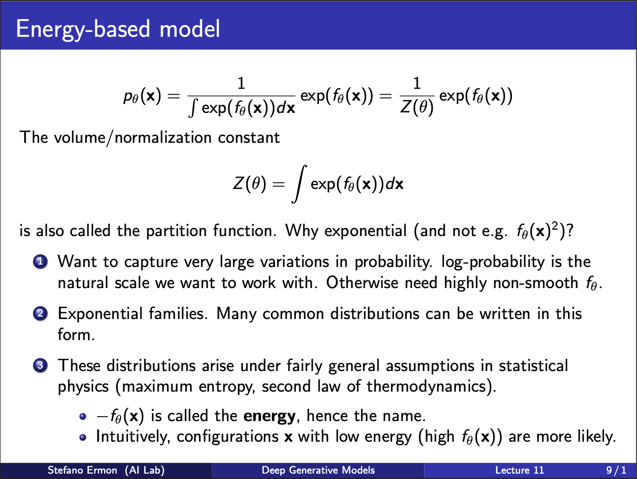
The most relevant way to define a model is to use an exponential function, where output of the net $\theta$ is raised to the exponents power, and divided by $\int e^{f_{\theta}(x)}dx$. The denominator term is called the partition function.

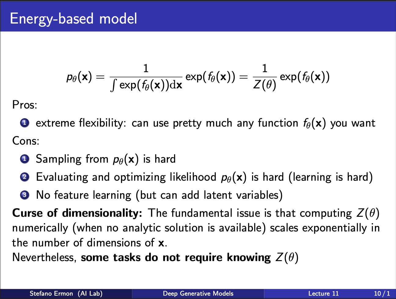
It is very hard to calculate this partition function in practice, especially when the input variable x can take many values, or is high dimensional.(For eg, x can be an image, even a image of $32\times 32\times 3)$ dimensions comes out to be 3072 variables, which makes computing the partition function to be a really difficult job). Also note that computing the partition function requires knowing the entire set of $x$, which is really difficult to do sometimes. Lucky for us, there are some tasks possible where we don’t need the partition function at all!!

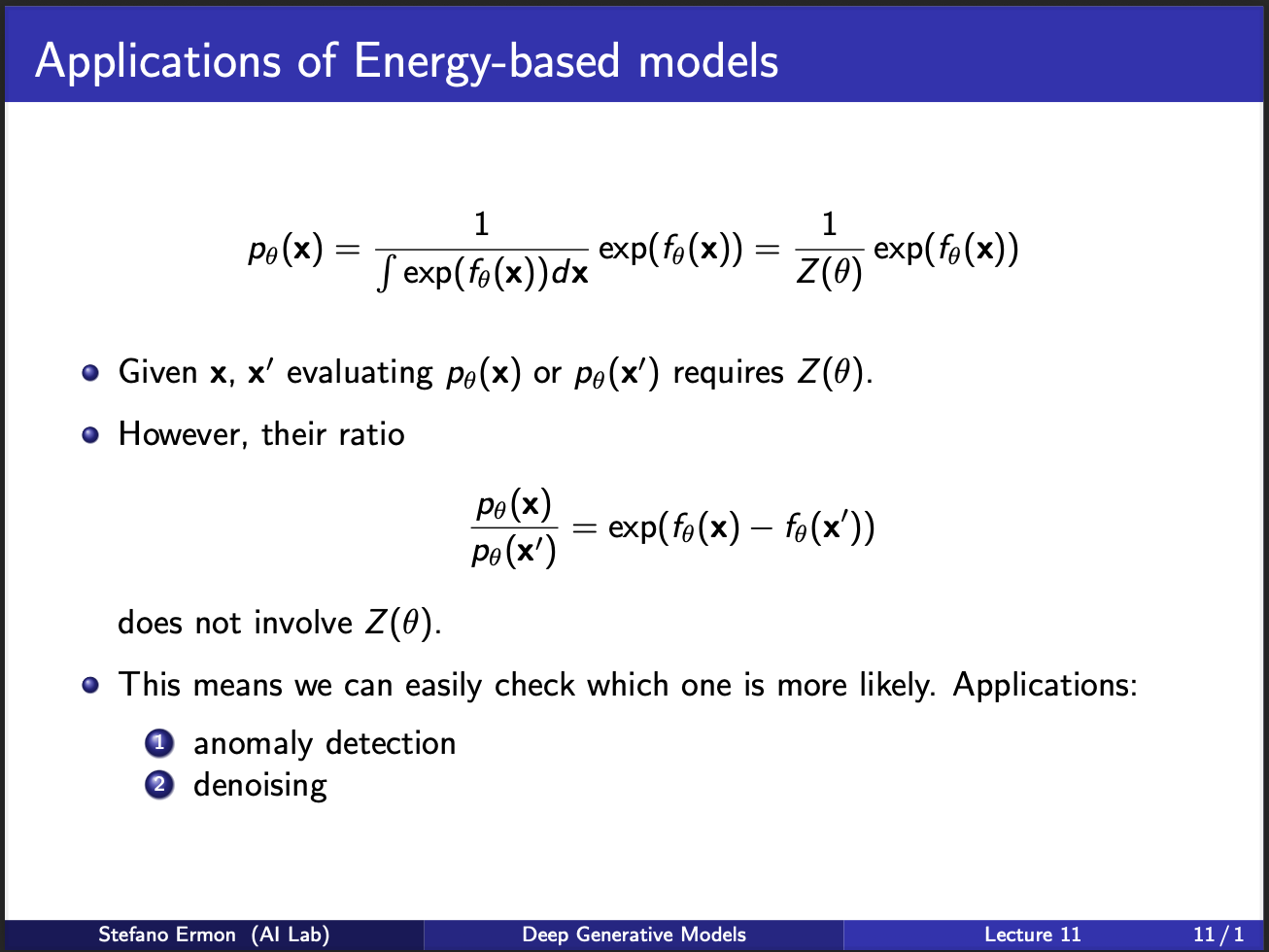
Let us assume we are given two samples $x$ and $x’$. Each of their likelihoods will involve the partition function. But, if you take their ‘ratio’ the partition function cancels out. So, what this means is that we can do tasks where we require `comparisons’ between relative occurences of two-samples, and not knowing their ‘actual’ probabilities. This has generally found application in LLMs, which are trained to model the relative ratios between different human responses.

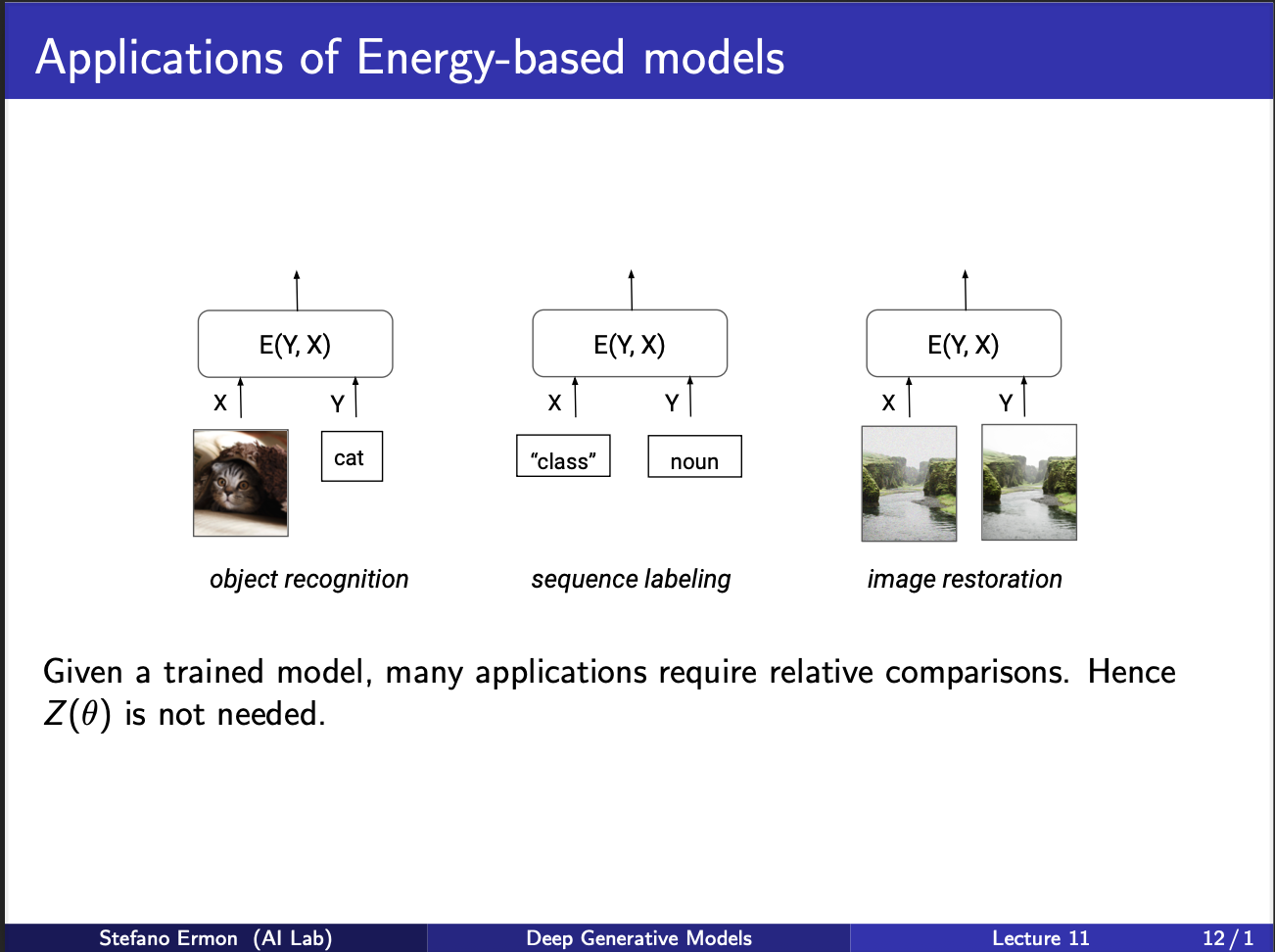
So consider the leftmost figure. If we are given image of cat, and a text caption saying it is cat, the resultant energy of the system is low (low energy means high likelihood). Similarly, we can think of other tasks where two images could be compared for eg, image restoration, which we discuss next.

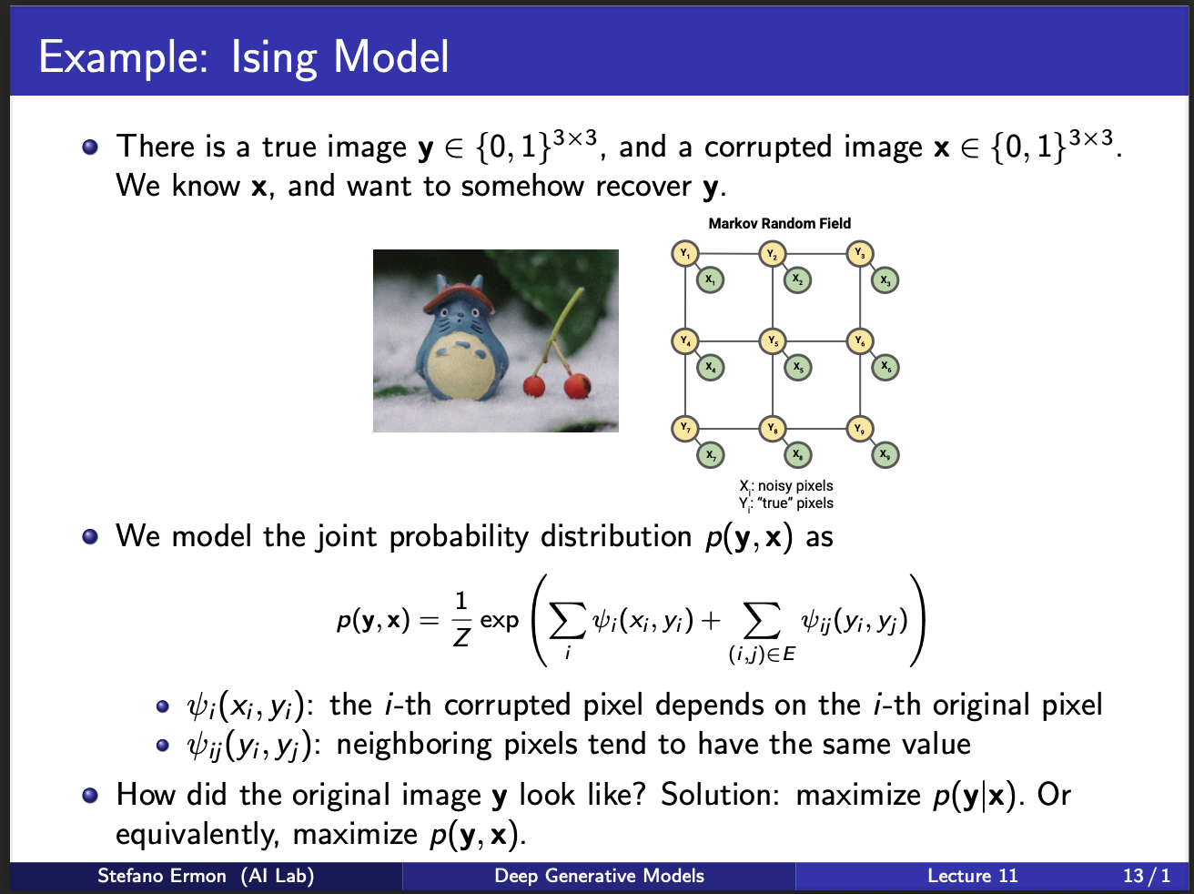
We shall now describe a kind of image denoising model called Ising Model. Assume that we are given a corrupted image $x$ and we wanna denoise it to a clean image $y$. So, we want to learn a discriminative model $p(y|x)$ or a generative $p(x,y)$. Modelling $p(x,y)$ is better since it also encodes the distribution of $p(x)$, as well as $p(y|x)$. A key property of ising model is that the output $y$ has each pixel either 0/1. This is discrete ising model. Continuous versions also exist, but that is not the subject of this lecture. So, the figure presents a $3 \times 3$ model. Note that, the $x$ input is the observed variable. We wanna learn a one-to-one mapping $<y,x>$, i.e. how does each y change give a particular x. Another constraint is that the nearby pixels of y $y_i,y_j$ should be smooth. These two terms are the constraints in the above equation. Note that $<x_i,x_j>$ is not modelled, because the input $x$ is already observed in practice.

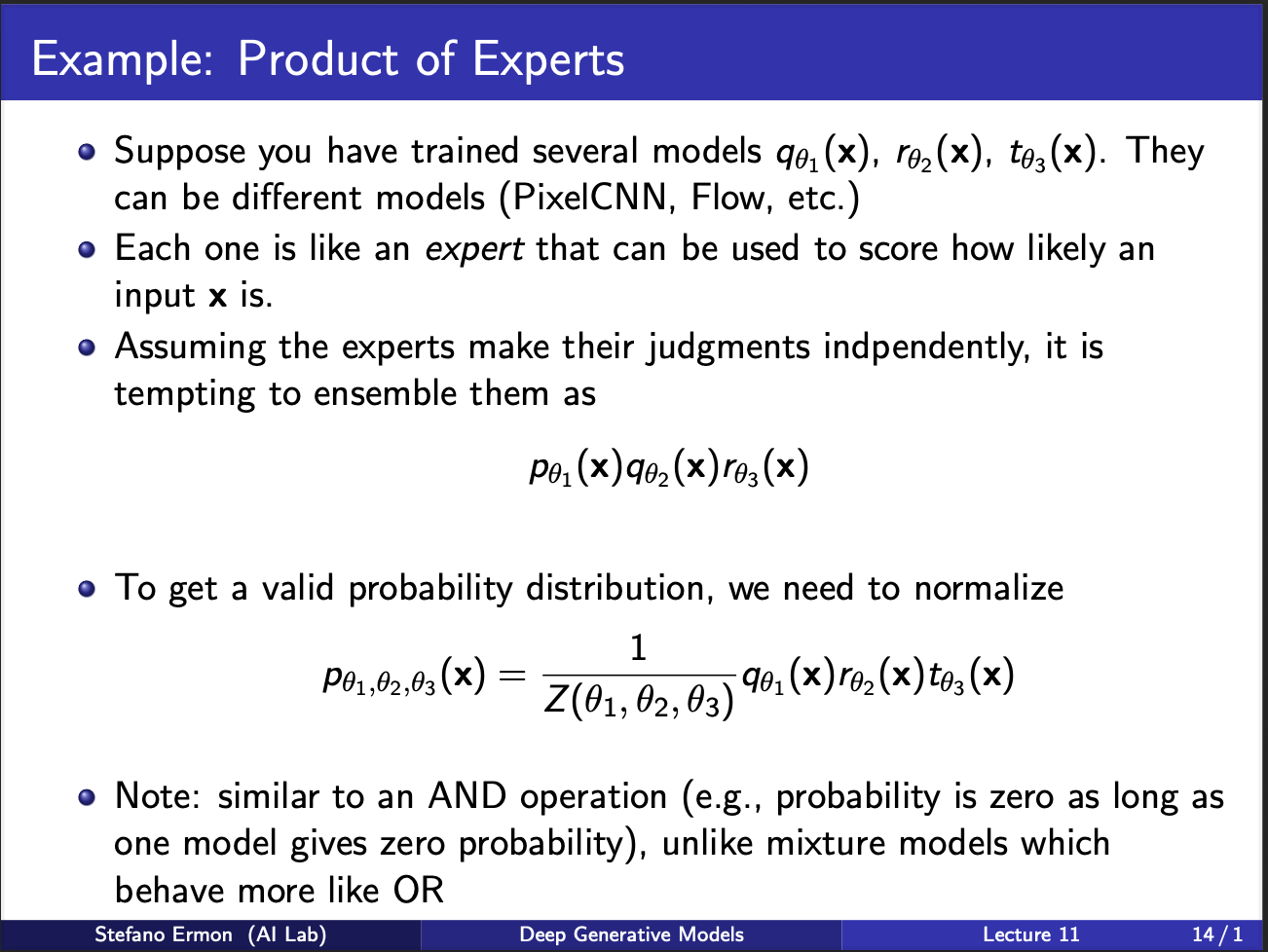
We shall now describe this idea of product of experts, which was originally invented by Geoff Hinton. Assume that you are given three models $p,q,r$, we want to somehow combine their predictions. The notion of combining is same as how democracy works: multiple people vote together to reach the consensus, and provided a large no of votes are captured, the individual bias, and noise gets cancelled out, and leads to a stable prediction. Therefore, the joint probability is given as a ‘product’ of these experts. Note that the notion of expert means that one model specializes in some task, another model specializes on another task etc. So when such a model seems an input x, it somehow has to decide, which of the models (p,q,r) will specialize in it. This requires a selection mechanism to be inbuilt inside the neural net.

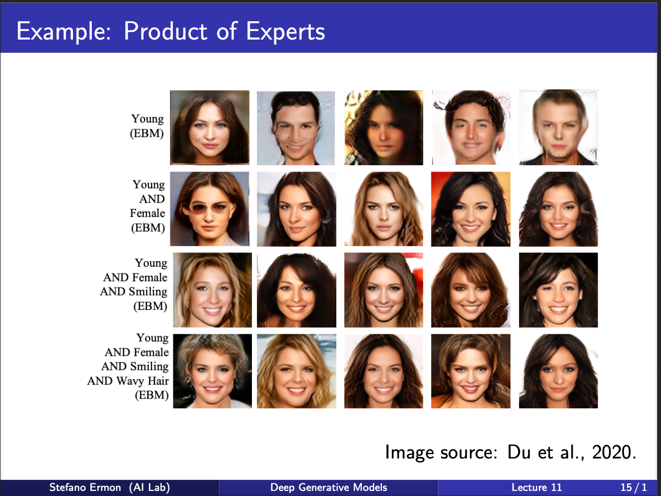
Let us now assume that such experts exist. For eg, one expert specializes in generating a woman, one specializes in generating young people, one generates smiling people etc. So, you can combine the outputs of all to generate a smiling young person (and they look very beautiful lol, i wish i had a girlfriend like that).

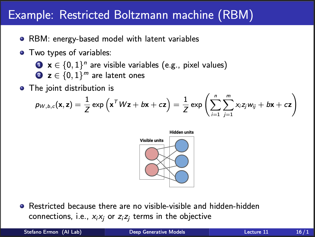
Geoff hinton could not stay still, so he invented another kind of machine called the restricted boltzmann machine. It contains two set of units, visible units and hidden units. Each input pixel is connected to N*N possible outputs, which means this would generate an image of size N by N. The boltzmann machine is called restricted because it does not connect input/output units among themselves. Neither does it consist of more hidden layers. The key reason behind this was that at that time, it was not clear how to train neural nets of more than one layer (since backpropagation was not invented yet).

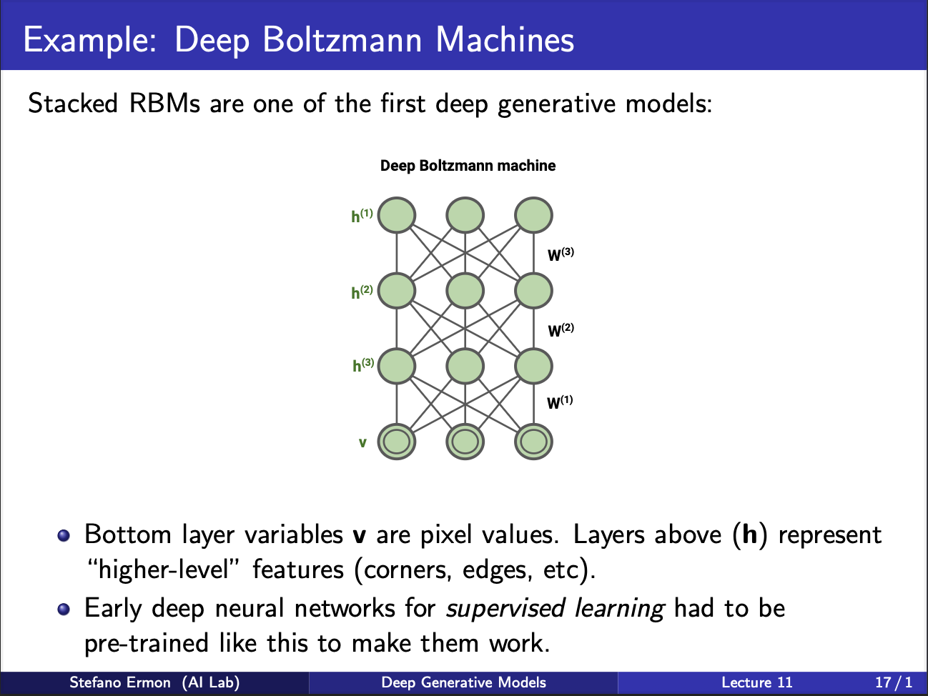
Another variant was deep boltzmann machines. It consists of multiple hidden layers. Training is done in a greedy way, first layer is trained, and frozen, the output features are used to train second layer and so on. Note that this procedure of greedy layer by layer training was ultimately replaced by alexnet in 2012, which used backpropagation to train the neural net end to end.

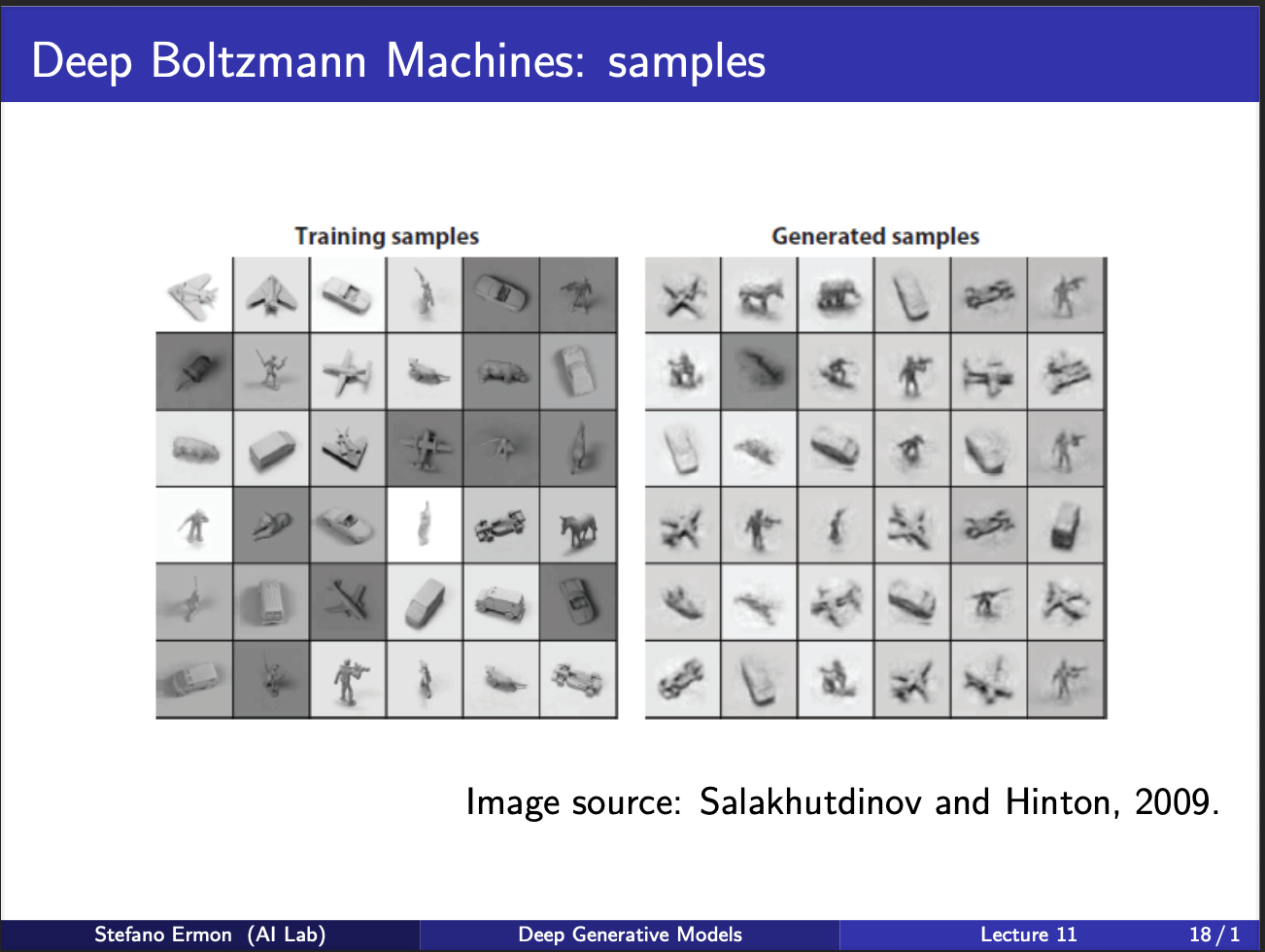
We can notice some shitty samples boltzmann machine generated. But at that time, it was a pretty big deal, to have a neural net generate new samples at all!!. Boltzmann machines have been succeeded with other class of generative models, but their key ideas still remain as fundamental guiding principles.

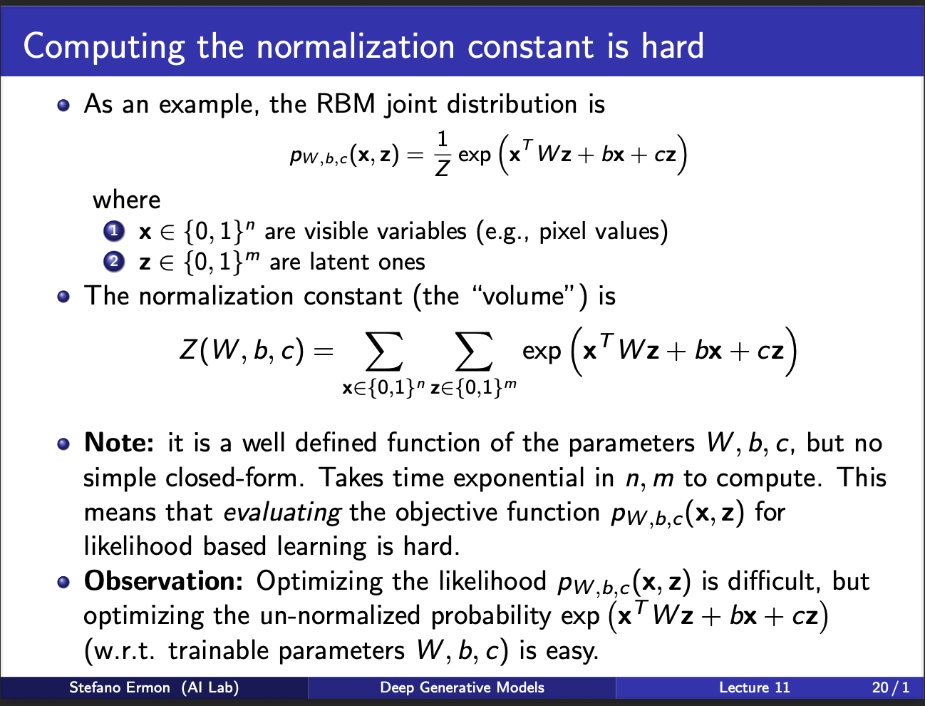
As an example, consider the joint probability distribution of a botlzmann machine. It looks very ugly, i know (sigh). However, it is time to focus on the denominator $Z$. Z is given by summing over all plausible values input x, output y. Evaluating this $Z$ is computationally very hard. However, note that if this denominator Z did not exist, we would have no issues, since the numerator consists of merely W, b, c. Alas, we can only dream, if only there was some way to get rid of this stupid z.

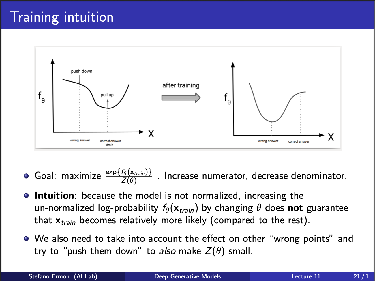
So, can we come up with a training strategy. Well to increase the likelihood, we wanna push the numerator up, denominator down. So, at the input x we are observing, we want probability to be high, and at “some other” points we want this probability to be low. ‘If’ we had some way of knowing these other points we would be in a good shape. So intuitively, there is a push-pull game going on. The probability curve $f_{\theta}$ vs input x, at the correct input x, should be high, and around it should be pressed down. In other words, x should function something like a hill, with many valleys lying around it.

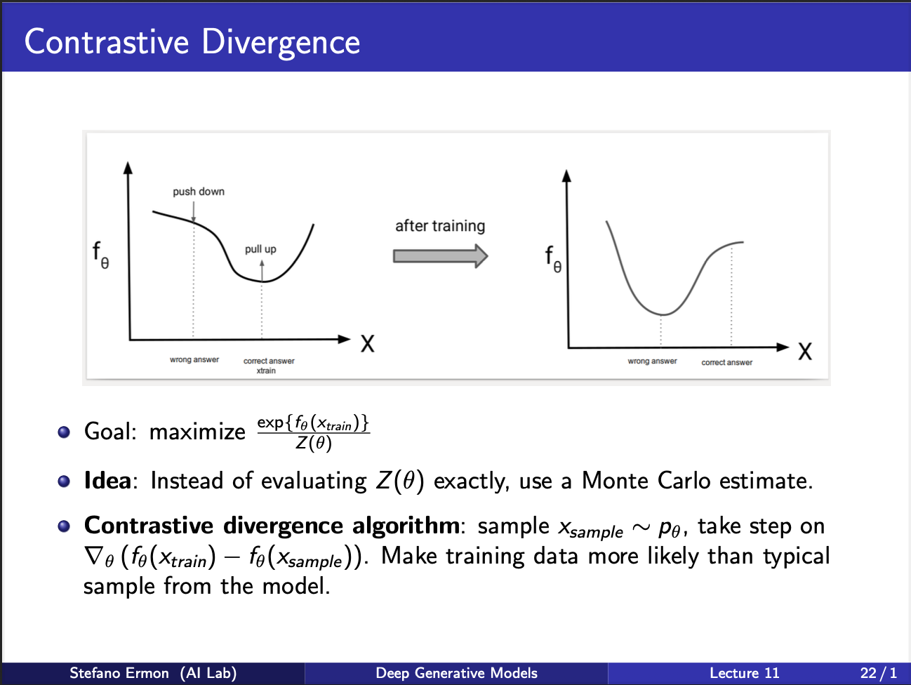
We shall now focus on the problem of how to know these “other points” we should minimize. Well the idea is “generate these other points from the NEURAL NET itself!!, and treat these samples as the negative samples!!”. Provided, you sample enough of these samples, you can make a good estimate of the gradient required to update this model. This idea is known as Monte-Carlo Estimate. There is no need to remember this fancy name, as long as you understand the key concept.

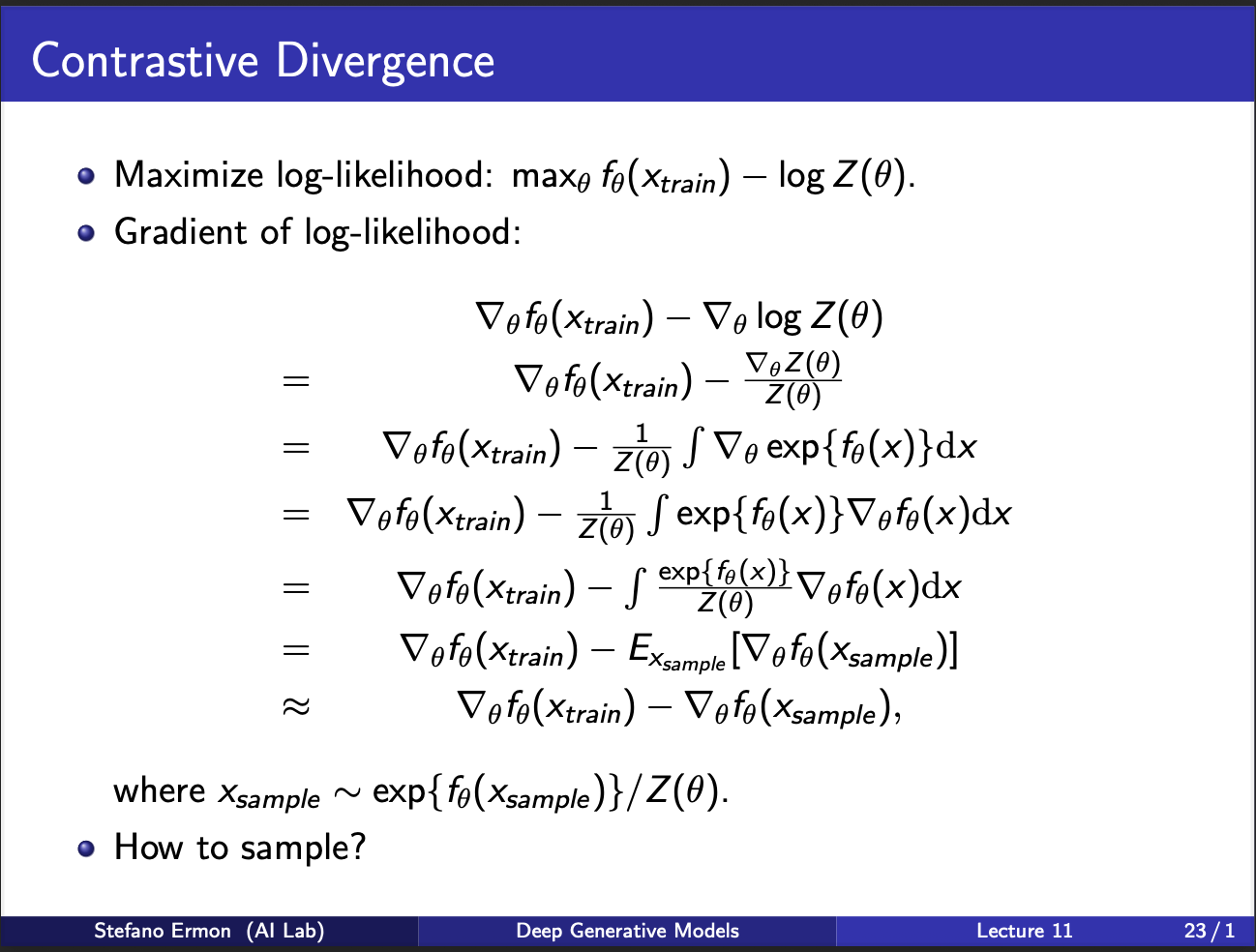
We shall now derive the expression of how to optimize a boltzmann machine. As you can see in the slides, it consists of two parts. First, is the gradient w.r.t input sample $x_{train}$. Next, we have to take a derivative of the partition function. If you track it closely, you can see that it can be written as gradient w.r.t some input $x_{sample}$, which is generated from the network itself. This leads us to the idea of sampling: how to generate these samples, which will ultimately be used to optimize the weights of the boltzmann machine?

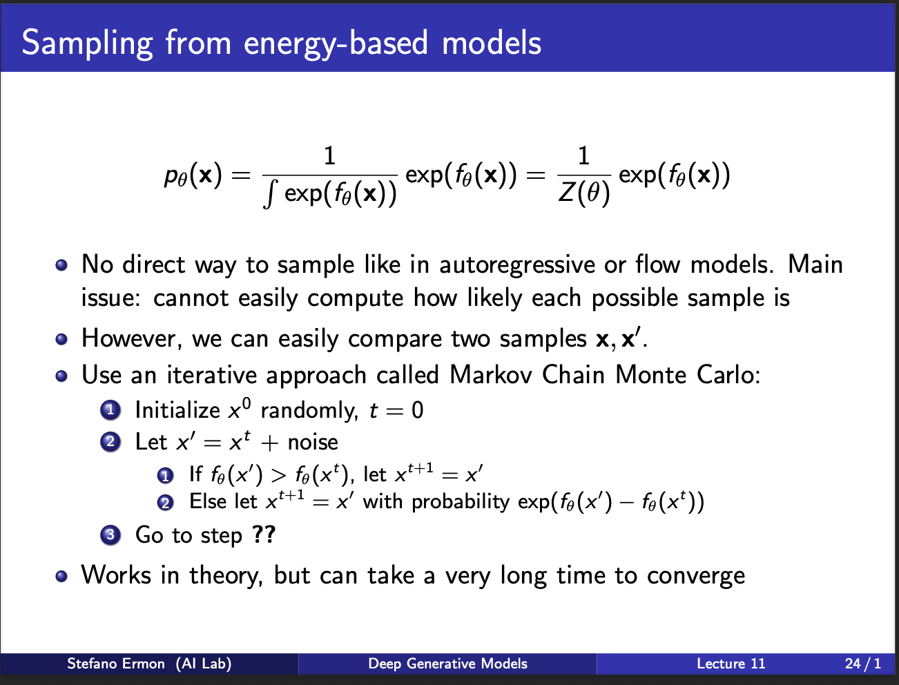
A closer look at the second term shows partition function in the denominator. As we discussed earlier, calculating it is computationally difficult!!. So how to sample lol :-). This leads to this idea of MCMC. The algorithm is to start with some sample $x_{0}$. We generate some noise, and compute a new sample $x’$. If probability of this sample is high, we choose it. If not, we choose it sometimes with a weight which is difference in the energy of $x_t$ and $x$. We can repeat this procedure for certain no of iterations. As you can imagine, it is extremely slow!!. For each iteration, you have to generate a lot of such samples, and then take a gradient. A core problem is this: 1) suppose you are standing at $x_{0}$, what will be the optimal direction to take a step during the sampling process. Is there something better we could do?

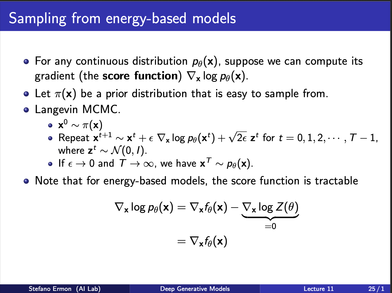
Well the idea is simple. You are standing in a probability space. You choose the direction, moving along which shall result in the max increase in the probability. This is known as a gradient. So, you can compute $\nabla p_{\theta}(x)$. And you know the next step you wanna take. So, it becomes easy to plug this in the MCMC equation. As you can see, you take the current $x_t$, move in the direction of gradient by a amount weighed by $\epsilon$, and sprinkle in some gaussian noise along the way. This is because, you want to explore the gradient space, and not converge to the same point after equal no of iterations.

The probability density function for an Energy-Based Model is defined as: \(\begin{equation*} p_{\theta}(\mathbf{x}) = \frac{e^{f_{\theta}(\mathbf{x})}}{Z(\theta)} \end{equation*}\) Where $Z(\theta)$ is the partition function, $Z(\theta) = \int_{\mathbf{x}} e^{f_{\theta}(\mathbf{x})} d\mathbf{x}$.We take the logarithm of the probability density function: \(\log p_{\theta}(\mathbf{x}) = \log \left( \frac{e^{f_{\theta}(\mathbf{x})}}{Z(\theta)} \right) \\ = \log \left( e^{f_{\theta}(\mathbf{x})} \right) - \log \left( Z(\theta) \right) \\ = f_{\theta}(\mathbf{x}) - \log Z(\theta)\) Next, we take the gradient with respect to the input data $\mathbf{x}$: \(\nabla_{\mathbf{x}} \log p_{\theta}(\mathbf{x}) = \nabla_{\mathbf{x}} f_{\theta}(\mathbf{x}) - \nabla_{\mathbf{x}} \log Z(\theta)\). Since the partition function $Z(\theta)$ is a scalar value that results from integrating over all possible $\mathbf{x}$, it depends only on the parameters $\theta$ and is independent of the specific input $\mathbf{x}$. Therefore, the gradient of $\log Z(\theta)$ with respect to $\mathbf{x}$ is zero: \(\nabla_{\mathbf{x}} \log Z(\theta) = 0\) Substituting this back into the equation yields the score function identity: \(\nabla_{\mathbf{x}} \log p_{\theta}(\mathbf{x}) = \nabla_{\mathbf{x}} f_{\theta}(\mathbf{x})\) Note that this a very powerful idea, since the gradient now becomes independent of the partition function. So, we dont need to estimate any negative samples from the network at all, during INFERENCE. However, training is still a bottleneck, since you still need to generate negative samples.

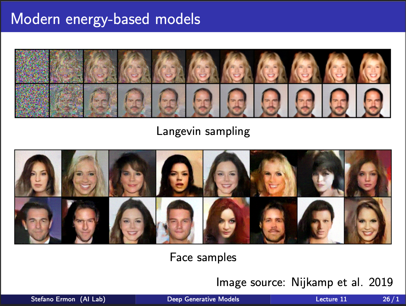
The figure shows some good faces generated via the sampling mechanism.

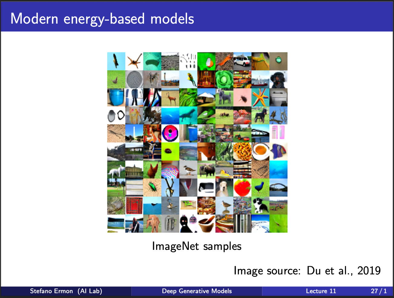
And these are some cute imagenet samples generated by some modern methods (not boltzmann machines). We are still left with a question: Can we build a generative model where we don’t need to sample negatives during TRAINING, and allow its optimization to be pretty fast.

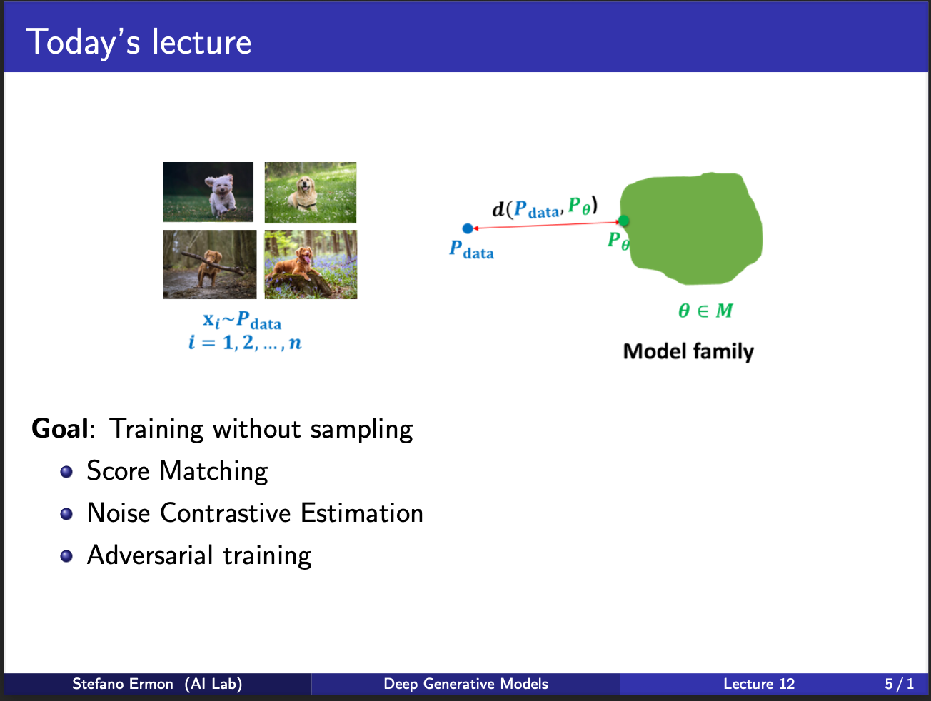
There are two kinds of methods which are relevant to training EBMs without having to sample during training. 1) Score Matching 2) Noise Contrastive Estimation. Note that I shall not focus on the adversarial training mechanism, since it faces a fundamental issue of mode collapse and is really not helpful to study.

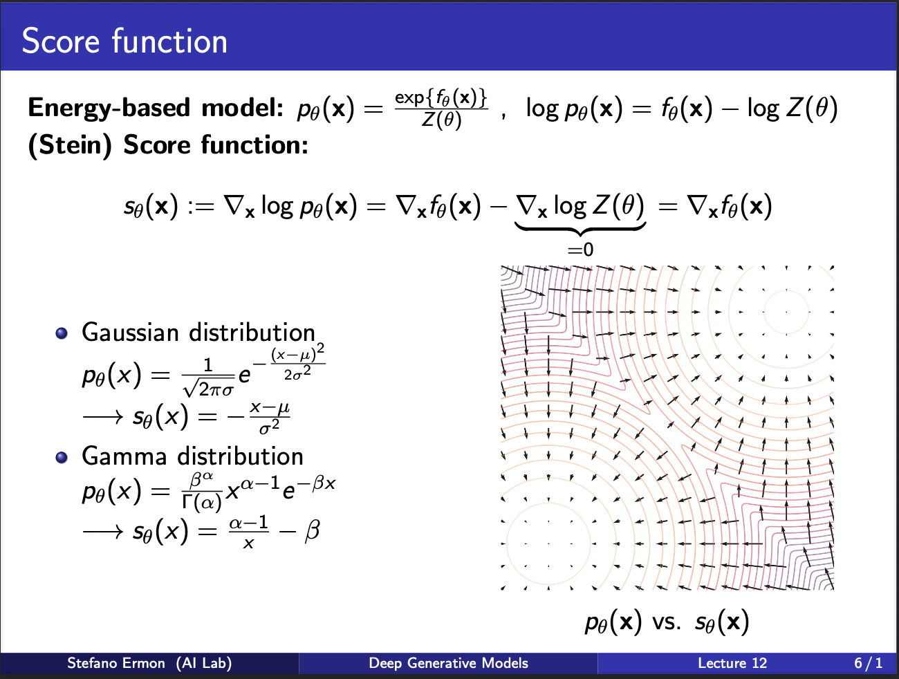
Recall that the pdf function is given by $p_{\theta}(x) = \frac{exp(f_{\theta}(x))}{Z(\theta)}$, where $Z$ is the partition function. The idea of score matching is to estimate the $\nabla_x p_{\theta}(x)$. Intuitively, this means that if we fluctuate the input x by certain amount, what happens to the output. So rather than modelling the probability, we model the gradient of the probability w.r.t input x. This results in a vector field. Consider the figure on the right, it contains several circles, which represent the $p_{\theta}$. Now, gradient of this is the arrows evident in the graph. So, we are trying to model this vector field.

One property to observe for this score function is that the gradient of the partition function comes out to be 0. This is because it only depends on $\theta$, and not the input $x$. This is a desirable property, because it means computing this gradient requires “NO sampling”, or computing a stupid partition function.

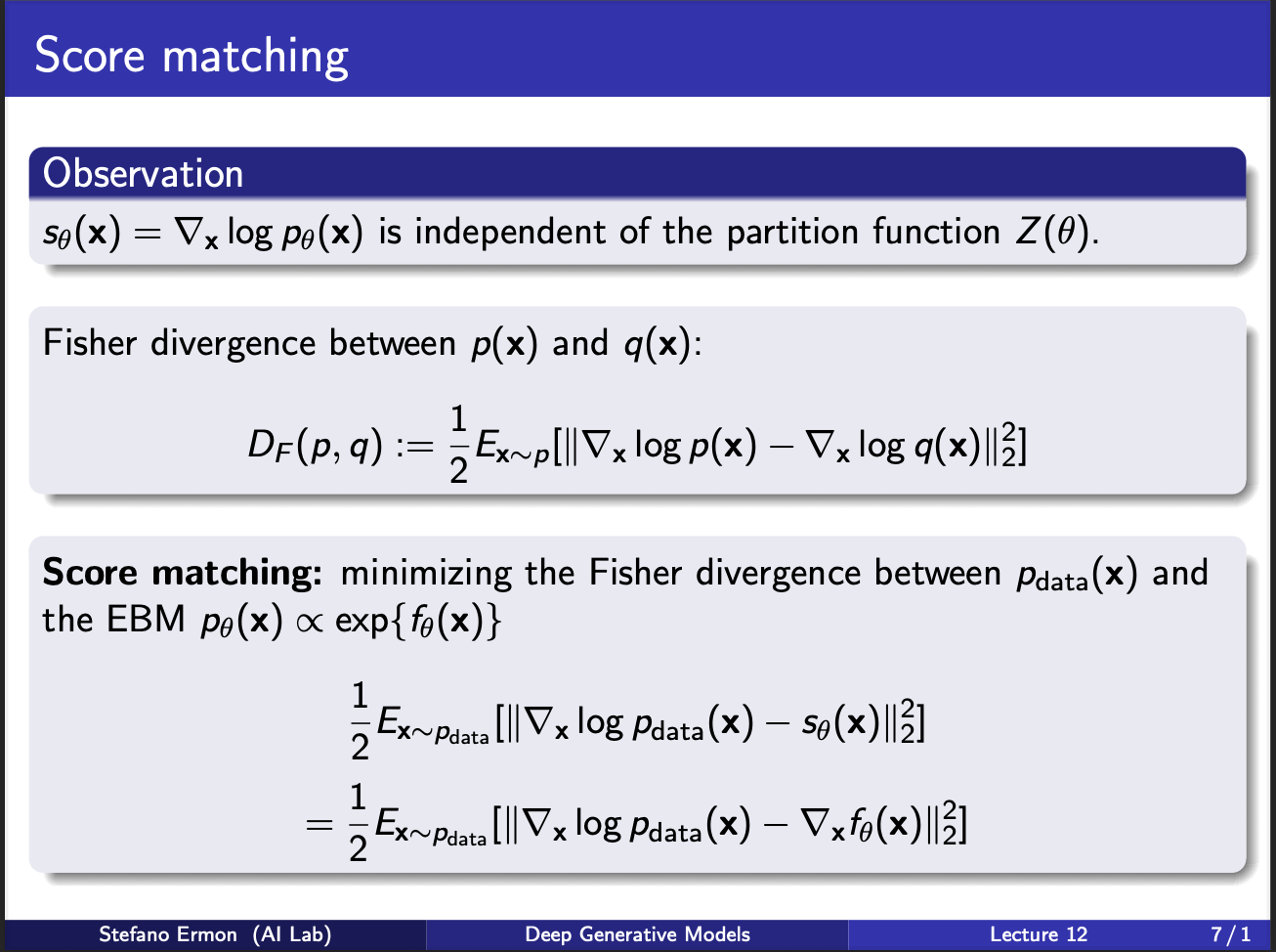
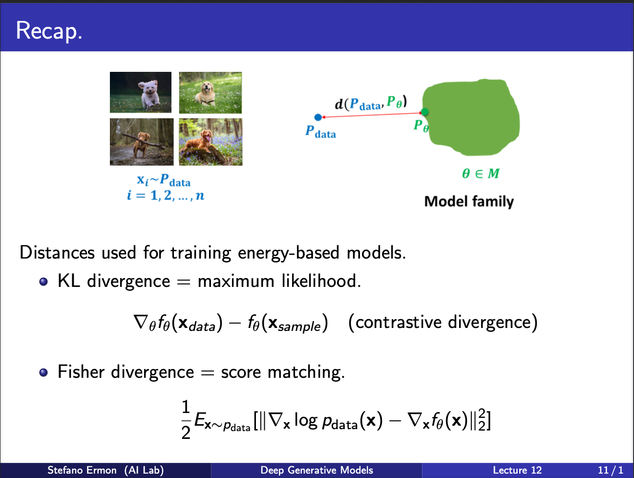
Next, we turn our heads to a measure of two probability distributions $p(x)$ and $q(x)$. Assume we calculate the score functions under both of these densities. We can define Fischer divergence as a measure of this distance. Note that the expression involves first sampling the input x from $p(x)$ and NOT q(x). The gradients are calculated at both the densities and subtracted from one another. Another thing to note, that this is NOT a symmetric function , i.e. $D_{F}(p,q)\neq D_{F}(q,p)$.

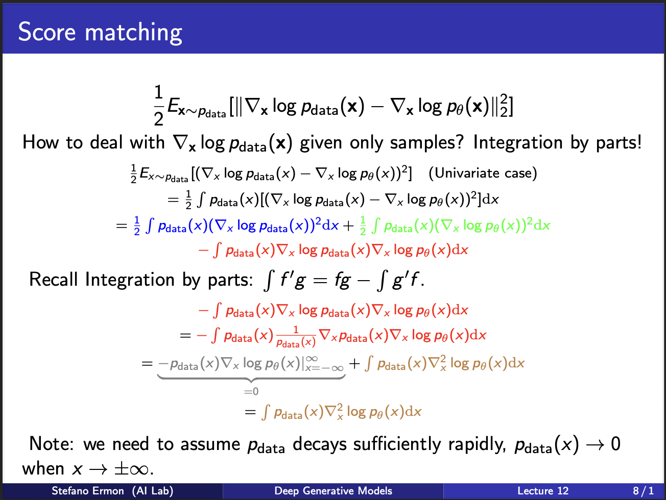
Next, lets take a look at some ugly math. Assume we are given many samples $x$. The score matching function can be broken into three terms which are blue, green and red. Take a closer look at the term in the red. You will see that we can use integration by parts there. Ultimately, it gives two terms. The left term is equivalent to $fg$ in the integration by parts, hence needs to be integrated on all plausible values of x. One assumption we make is that $p_{data}$ tends to $0$ at boundaries, which will enable this term to be 0. So this red term becomes simplified.

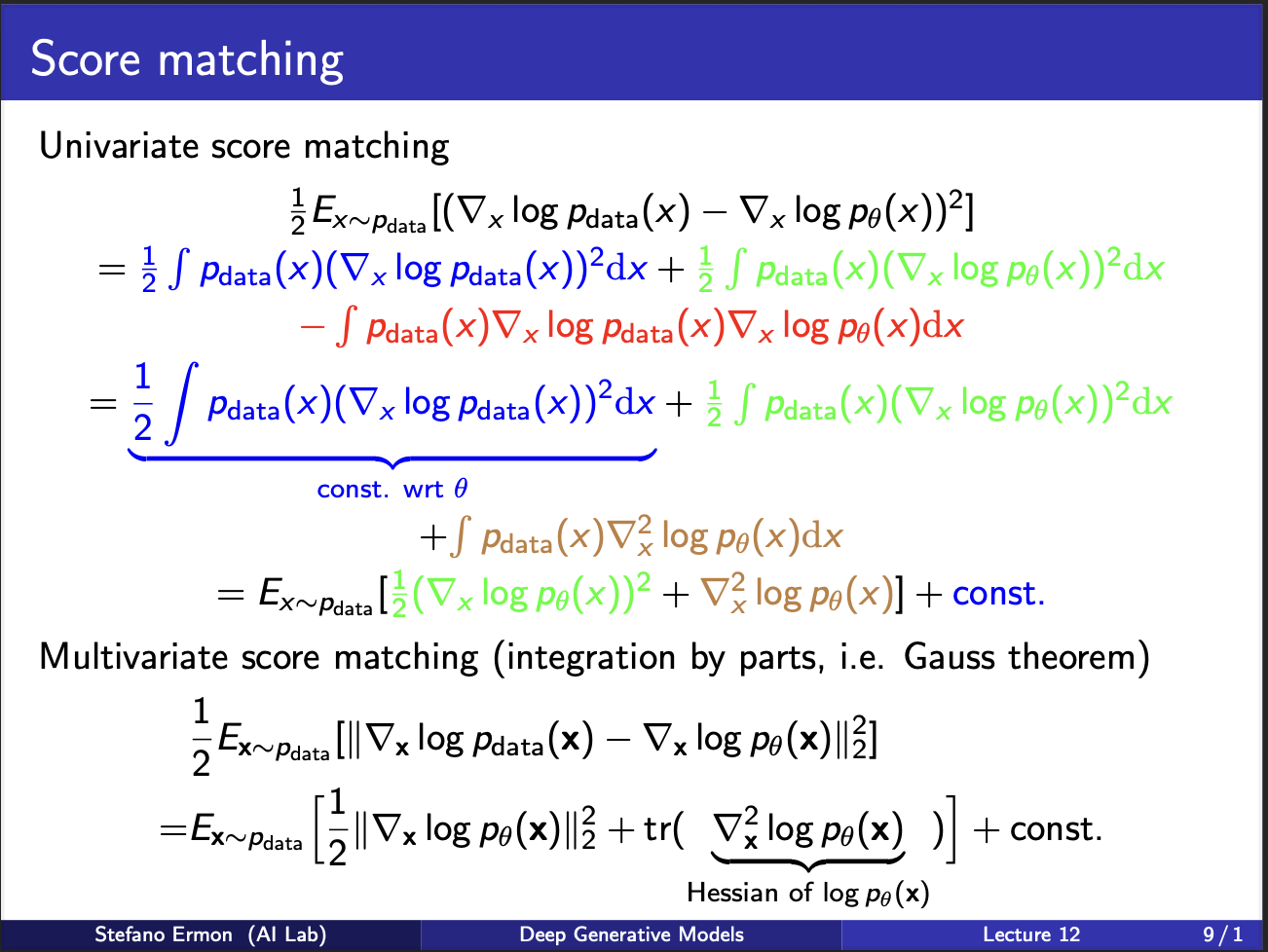
Let us look at ugly math some more lol. The score function consists of three terms (with red term) simplified. The first term is something with does not depend on $\theta$ at all, so we dont need to optimize it. Let us assume it is some constant. The green and brown terms contains $\nabla p_{data}$ , we can bring that outside, and take an expectation. Note that the final expression involves a gradient of log probability function, and second term involves a `second order gradient’ (which is also known as hessian)

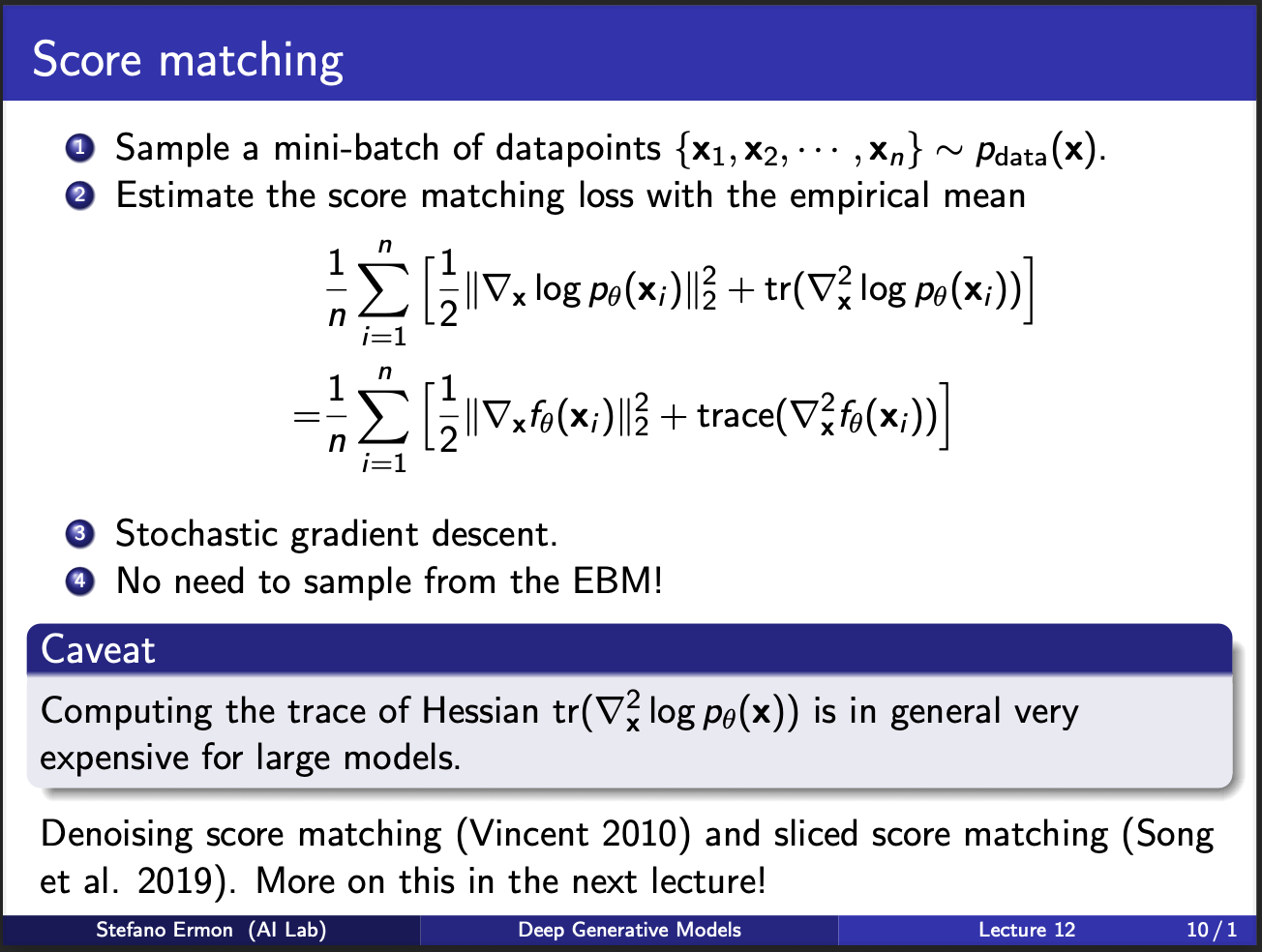
The algorithm of score matching then becomes pretty simple. First, sample n samples from the true data disstribution, and n from the noisy distribution which is already known. Then compute the mathematical term which is given, and we will have our answer. Now, the issue appears in estimation of this hessian. If $x_{i}$ is 100 dimensionsal, jacobian will be $100 \times 100 = 1000$ and hessian will be $1000 \times 1000$, therefore the memory will quickly explode for $n$ samples taken at a time. Therefore, it means that computing the trace function is a key `problem’ in the score matching. Is there a way to get rid of it? We shall discuss this later in this post.

Recall till now, we have understood the mechanism behind score matching function. Its key problem had been that the hessian had to be computed. Next, we shall turn our attention to Noise-Contrastive Estimation :-).

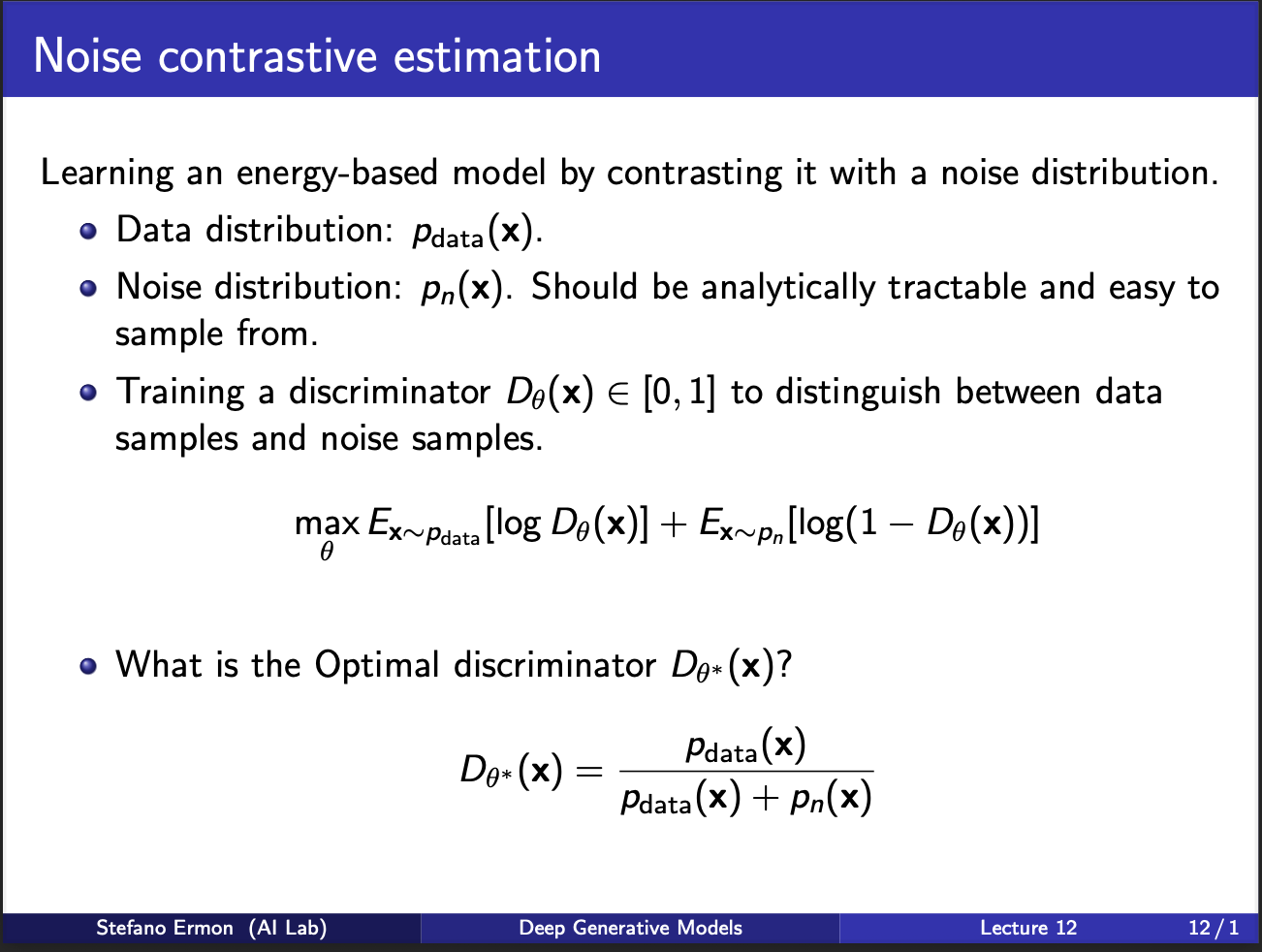
Well the key idea goes as follows: you don’t know $p_{data}(x)$ in advance. But, you can assume a noise distribution $p_{n}(x)$, from which you can sample a noisy sample. Then, imagine training a neural net to look at real sample, or noise sample, and predict whether it is real or noisy. Let’s call this as a “discriminator”, parameterized by $\theta$. The aim is that if sample is real, discriminator should output a high value, otherwise it should output a low value. An ideal discriminator, will be the one which can separate $p_{data}$ from a mixture of distribution $p_{data} + p_n$.

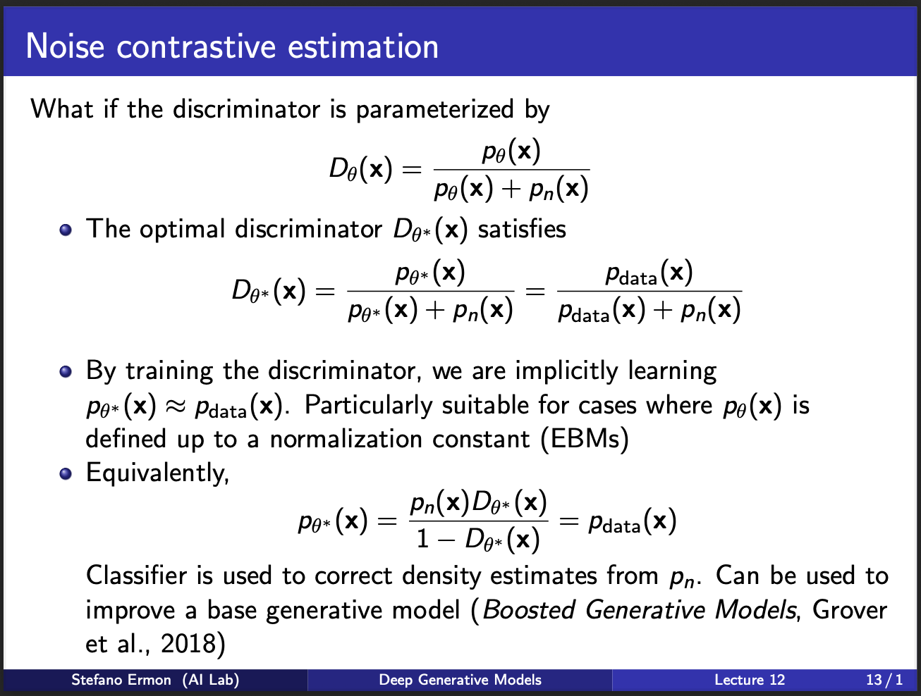
So we assume that the optimal discriminator is parameterized by $\theta^{*}$. While we are training discriminator, we are implicitly learning to match the distribution of the true real data.

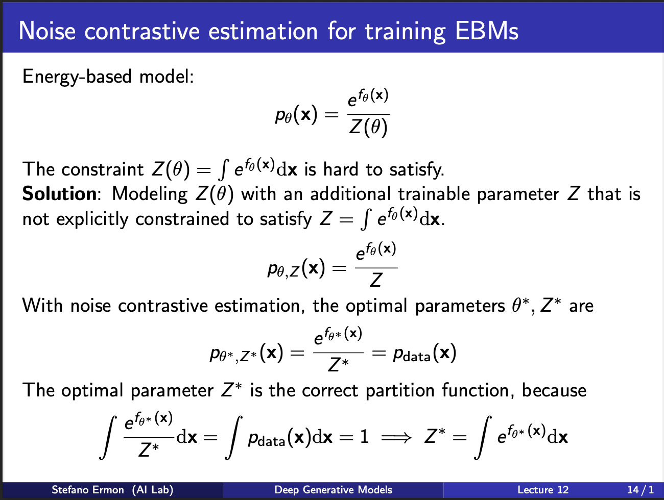
Recall that a standard EBM contains a exponential function divided by a partition function. But computing partition function is very difficult. So one idea is : “learn” the partition function also. In simpler terms, we can model a joint probabilty distribution $p_{\theta, z}$, which contains learnable parameters $\theta$, as well as $z$.

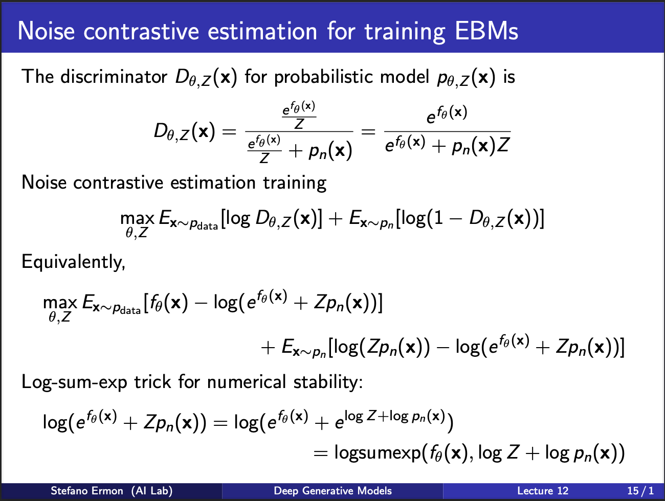
We can compute the expression for the discriminator $D_{\theta, Z}$ by incorporating the probabilistic model $\theta$, $z$, and pre-known noise distribution $p_n$. NCE loss requires training discriminator with the expression above.

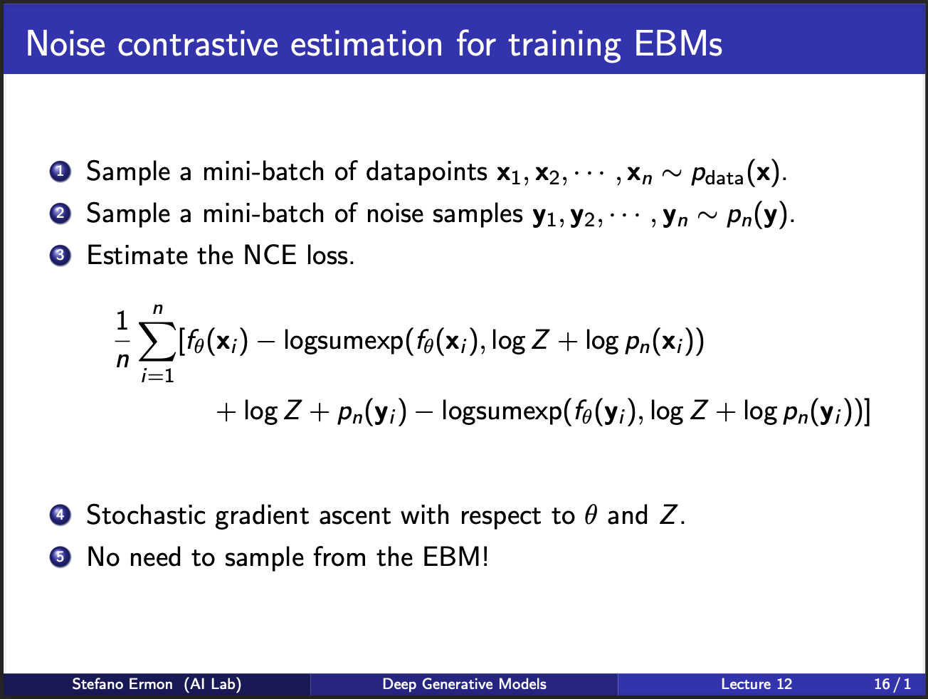
The algorithm then becomes : sample some data points from true distribution, some from noisy distribution, and compute the nce loss. The parameters are then updated via standard stochastic gradient ascent. Note, that this step does not require sampling from the EBM!!. If you zoom back , this algorithm points to something weird: you can add noise, and classify it. Somehow, it allows us to get rid of the partition function, and just learn it!!. Furthermore, there is no stupid second order derivative here, so thats pretty cool :-).

However, note that we only classified a given sample as belonging to some real data/noise. Could we build a better model, where we also estimated the “amount of noise” we added to a sample? Hmmm, it seems we are gradually building towards diffusion models lol.

At this point, lecture 13 started. So, i had to actually go into the ppt, and see what dr. ermon was saying :-). So thankful that stanford guys provided the notes. Really beneficial for a dumb duck like me.

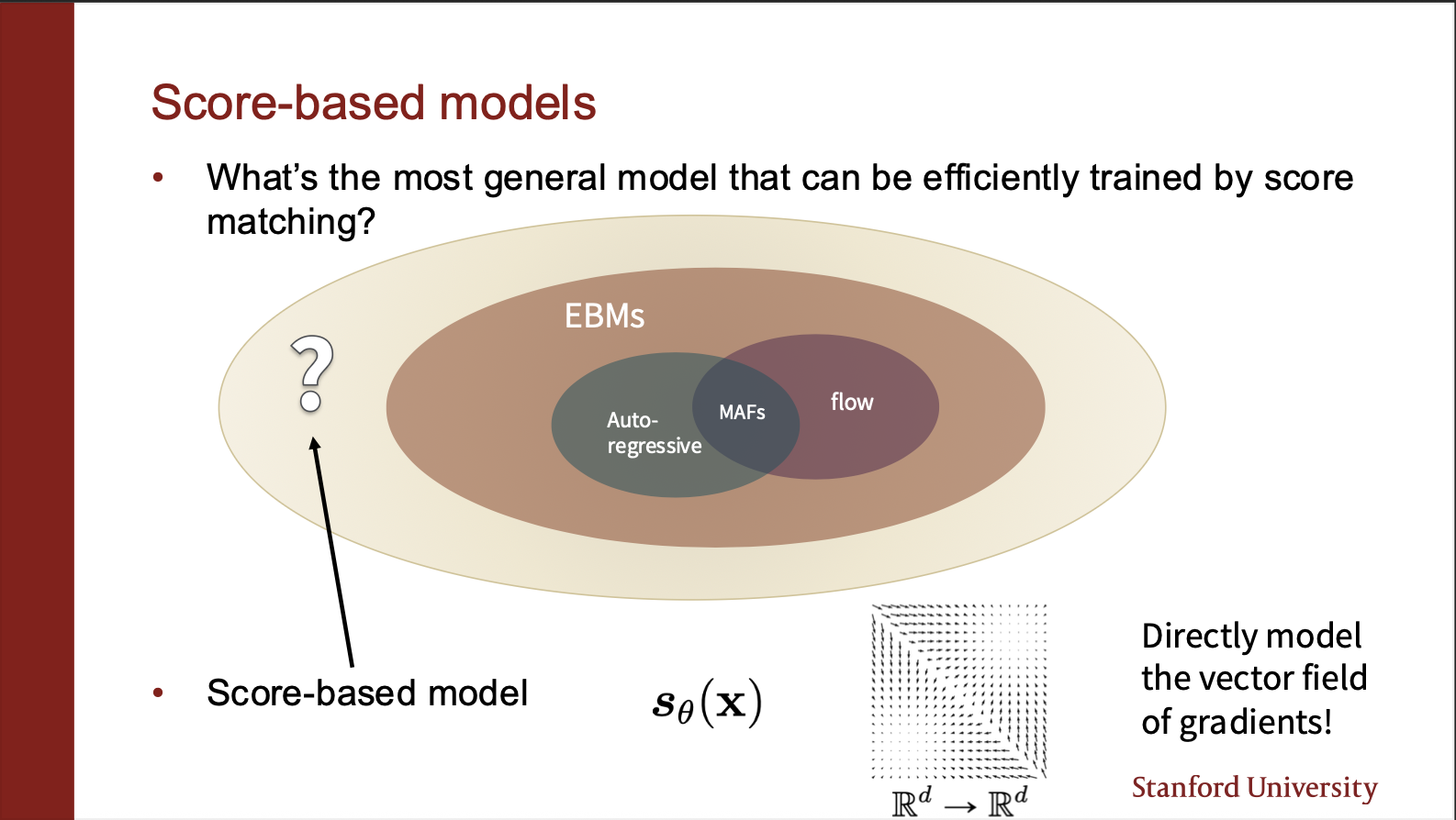
We can now start imagining a plausible universe in which the score matching models lie. They are generalizable over EBM’s because we can in theory use score matching to even train a Flow model, etc.

Let us now focus on building some intuition of score matching. Assume we are given a data generating function (which is a mixture of two gaussians), and we draw some samples from it. Note that the density in one gaussian is more, as compared to another, i.e. we give more “weight” to one of the gaussians. We can sample iid samples in this distribution, to get two clusters , one of which is more spread than the other. We wanna somehow compute the gradient of the likelihood of these samples, and compute a vector field. This vector field should match the field of the mixture of gaussian (on the left). This notion is known as “score matching”.

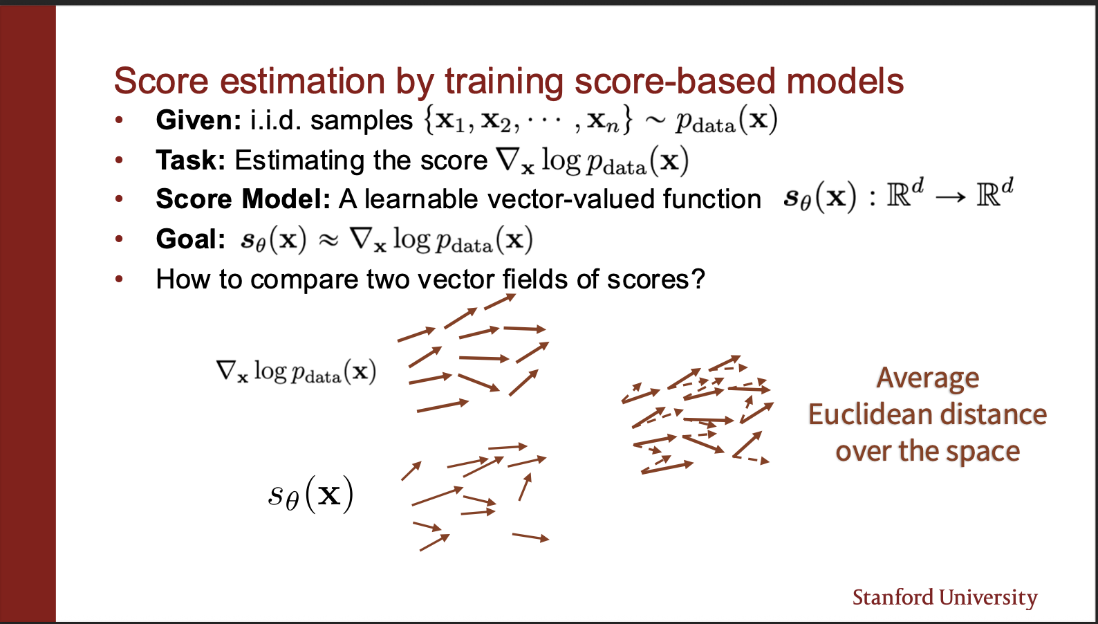
So let us imagine that we have a ground truth vector field, and a field predicted by the score function. We can align these two, and measure the “angular” distance between them. This will give us an approximation of how close we are to the real distribution.

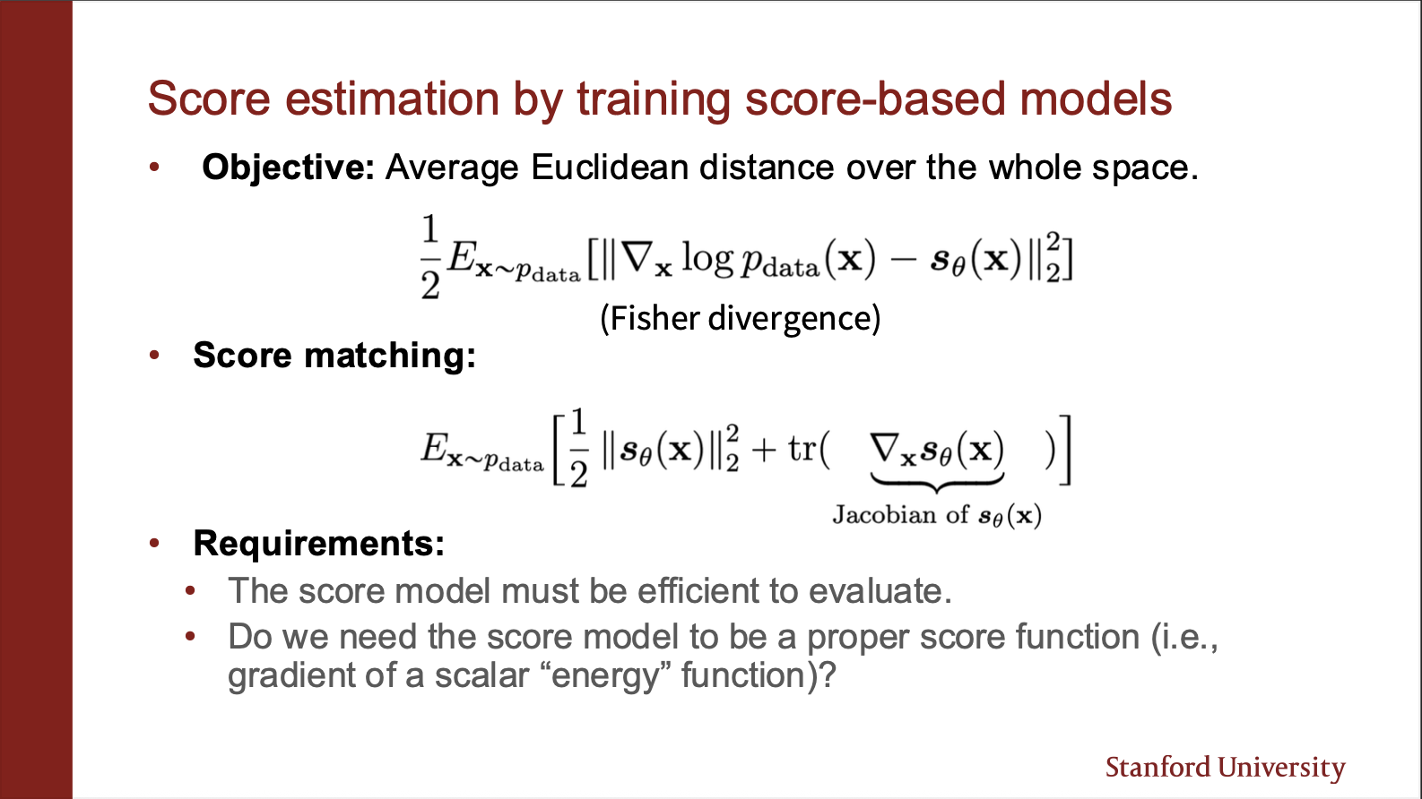
The $L_2$ norm between these distributions is known as the fischer distance. Unfortunately, this thing depends on $\log p_{data}(x)$, which we don’t know. Luckily, we can simplify this as the score matching equation, which only involves $\theta$. The key bottleneck comes from the jacobian part. (note that hessian is second order derivative, jacobian of a jacobian gives a hessian.)

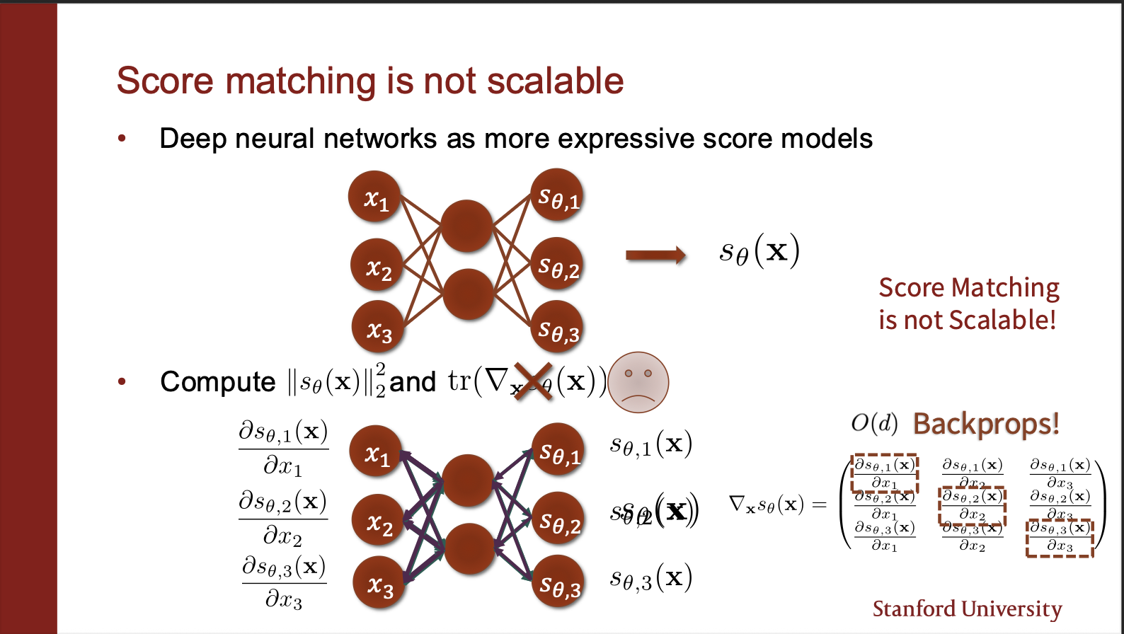
We could parameterize the score network as a neural network. However, computing the jacobian is intractable. Consider the output neurons modelling $s_{\theta, 1}$. We need to compute the trace of the jacobian, i.e. how does the value of first output neuron change if first input neuron is changed. Similarly, we have to do this for other $d-1$ dimensions of the input. Hence, we need O(d) backward passes.

Now, if you were looking closely, you will see, we could just perform a single backward pass. Will that work? NO. Consider second input neuron. Fluctuating that should not impact any other output neurons other than second one. Therefore, we need to make sure that gradients of other output neurons are not impacting the second input neuron. That is why we need O(d) backward passes. This scales with the number of input dimensions of x, which is not really a good option. Can we do better, say somehow compute the gradients in only a single backward pass?

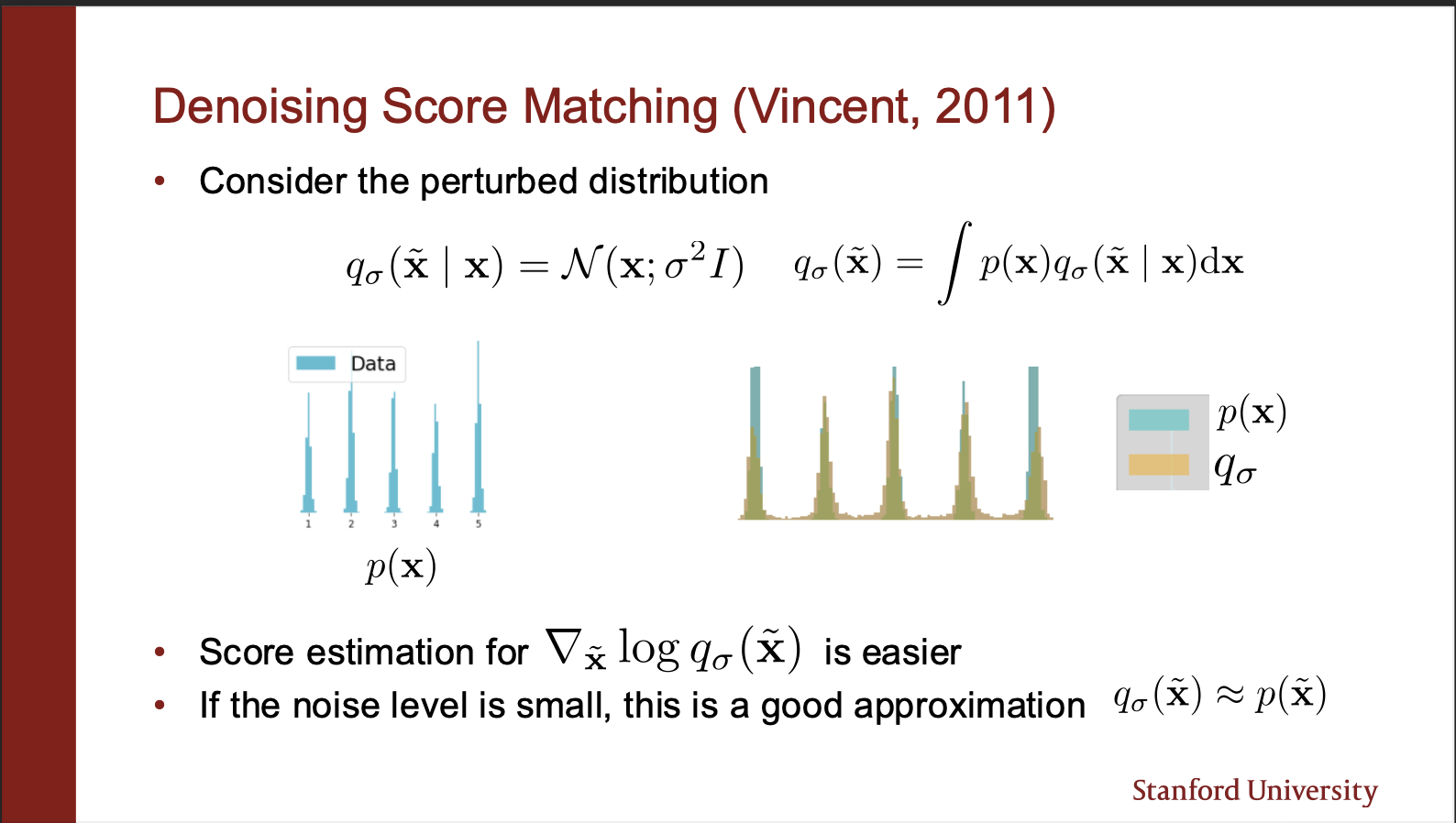
A way around this problem was invented in 2011, under the idea of : denoising score matching. Let’s say we are given a ground truth probability distribution $p(x)$. It says that we can perturb the clean images by some slight noise (for example a gaussian kernel, with very low variance). Let the perturbed distribution be called $q(x)$. So rather than estimating the score of $p(x)$, it is far more computationally efficient to calculate the score of $q(x)$. How? Well that proof requires some math, which we will discuss next.

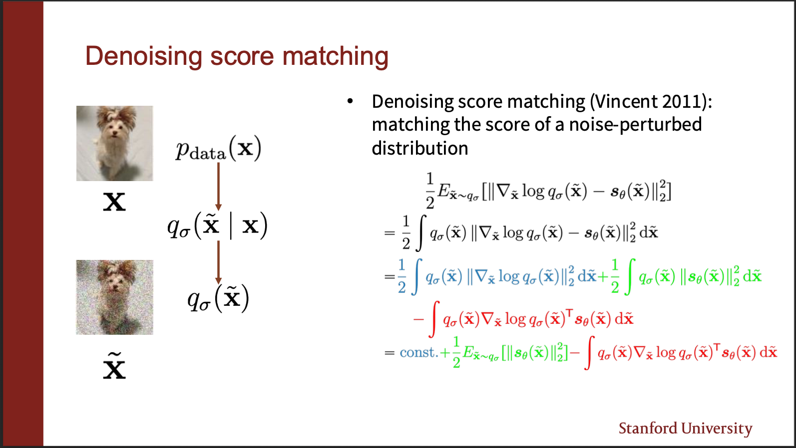
As before, if we simplify the score function, it appears to have three terms. First term (the blue part), does not depend on the parameters $\theta$, so it can be assumed to be constant. So let us only focus on the green and red term.

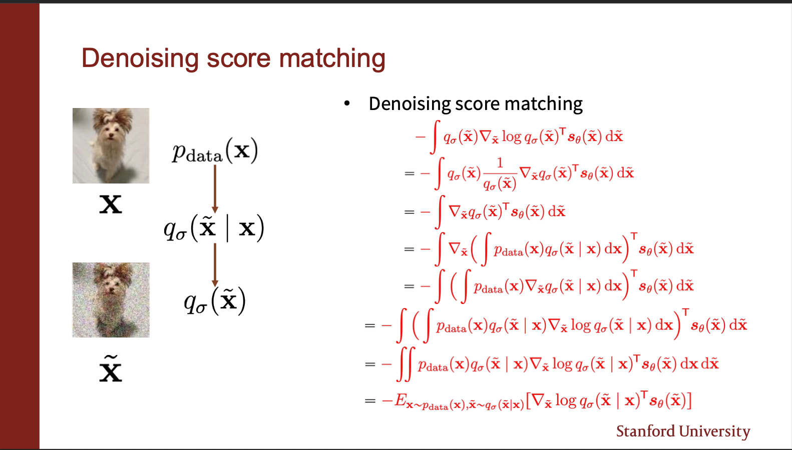
The second term contains $\nabla_{\tilde{x}} q_{\sigma}(\tilde{x})^T$. Now remember that there are several possible inputs x, which are corrupted by a kernel q, to compute $\tilde{x}$. Therefore, this term can be written as a product of probability of sampling $x$, and the probability of generating $\tilde(x)$ `given’ the input x. We can integrate then by summing over all the plausible $x$. The gradient outside depends on $\tilde{x}$, so it can be brought inside the expression. So we finally get a term which contains the expectation. Remember this is the simplification of the RED term.

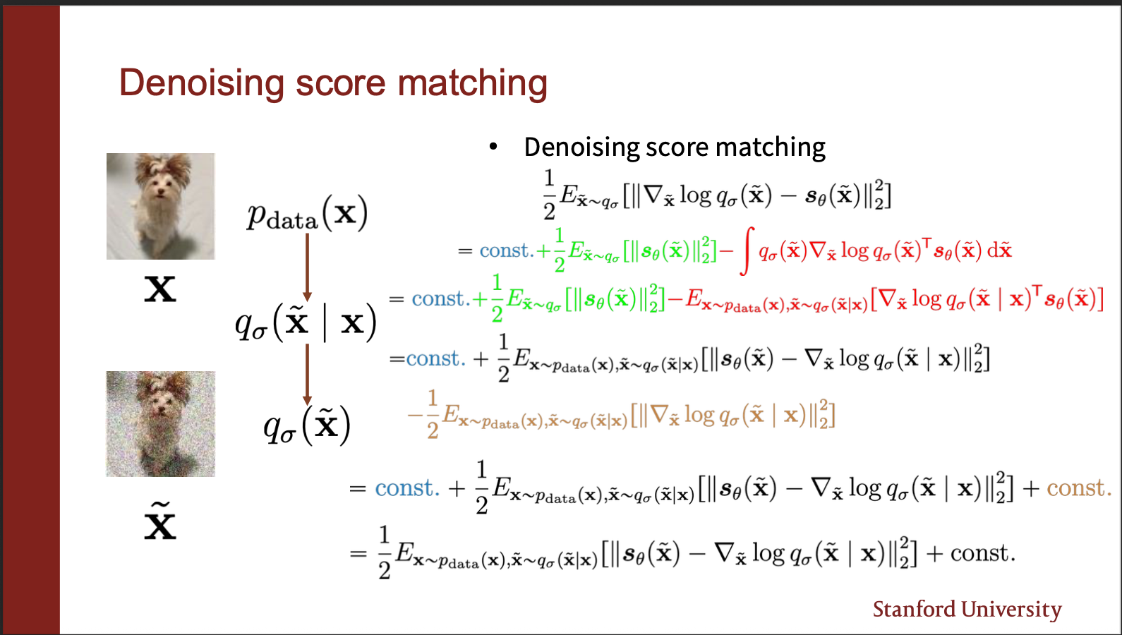
You do a bunch more math, and end up with the final term, which i will explain next. I think while it is important to derive on your own, the key message is: noise the input, and learn a score network that mimics the vector field of the noisy distribution.

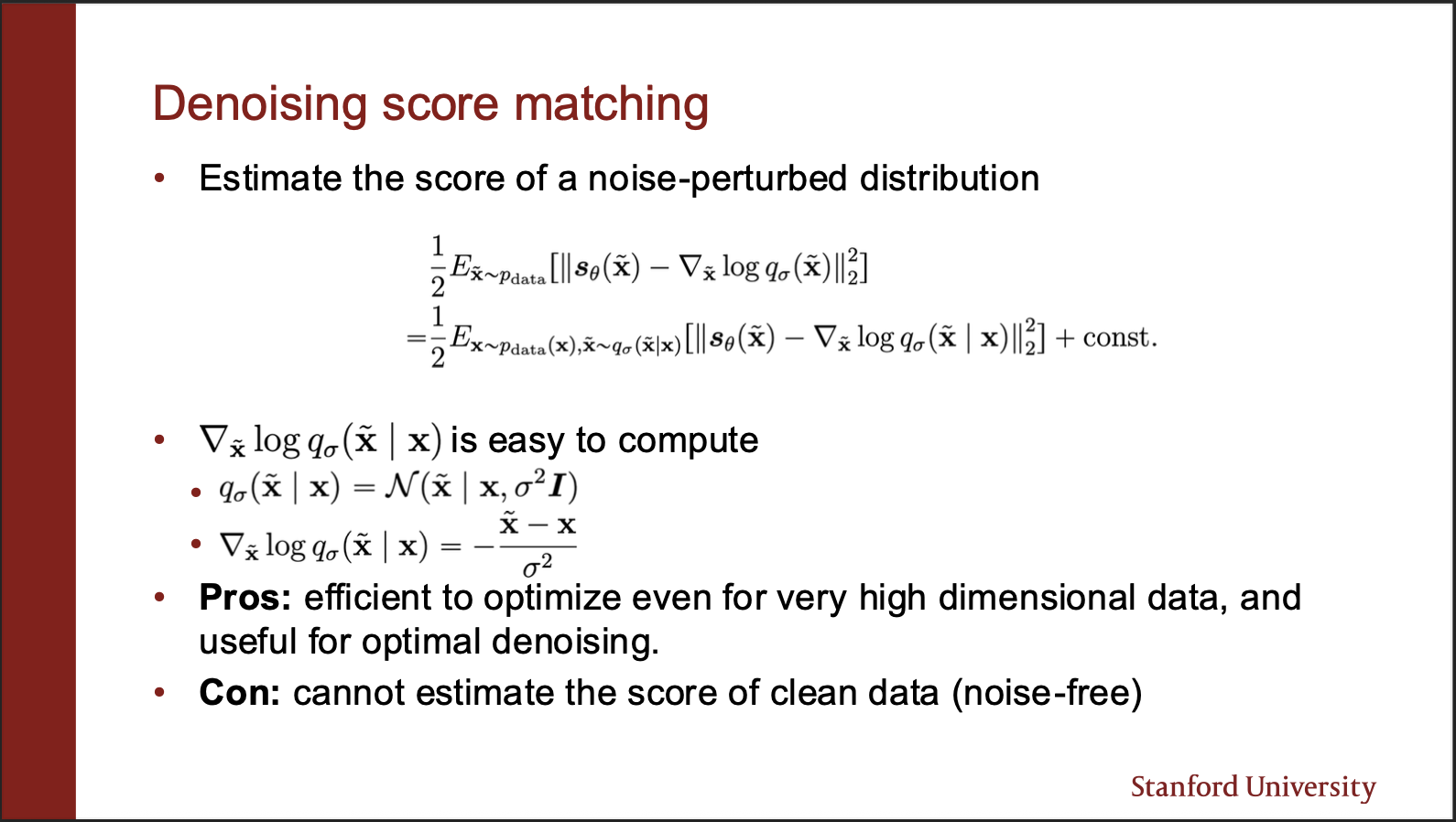
The final equation comes out to be very elegant. The first term is just the value that the score network predicts. The second term is the gradient of log probability of noise sample conditioned on the true sample. This is nothing but just a gaussian noise which we added, whose mean and variance are already known. So the gradient is simply the negative of difference between noisy and clean sample, divided by the variance.

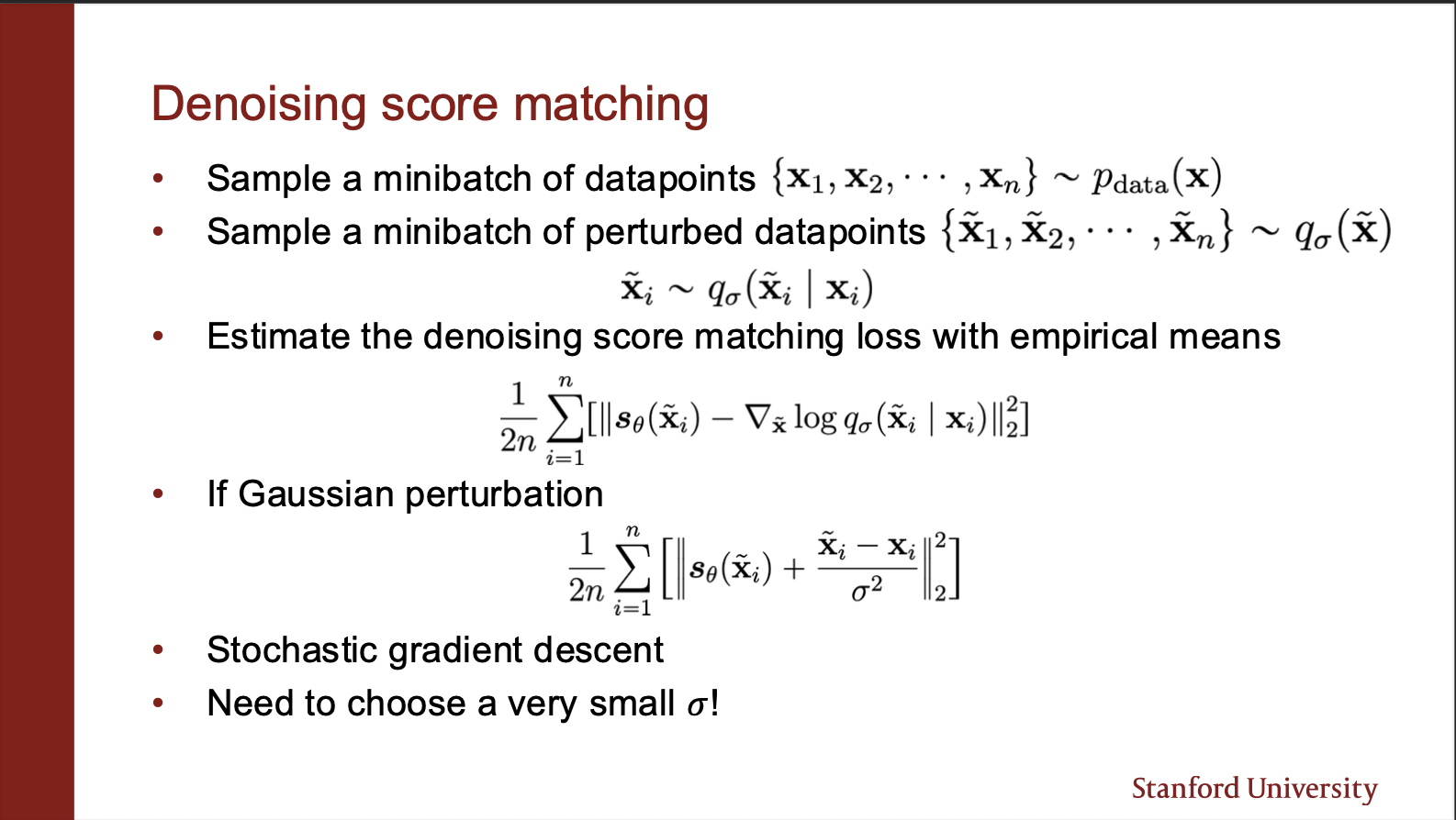
The denoising objective then becomes pretty sleek: you sample a bunch of datapoints, and perturb each of them under a noisy kernel (gaussian in our case). Then you compute the score matching function, and make a gradient `ascent’. One important point here is that the variance of noise added should be pretty small for this method to work well.

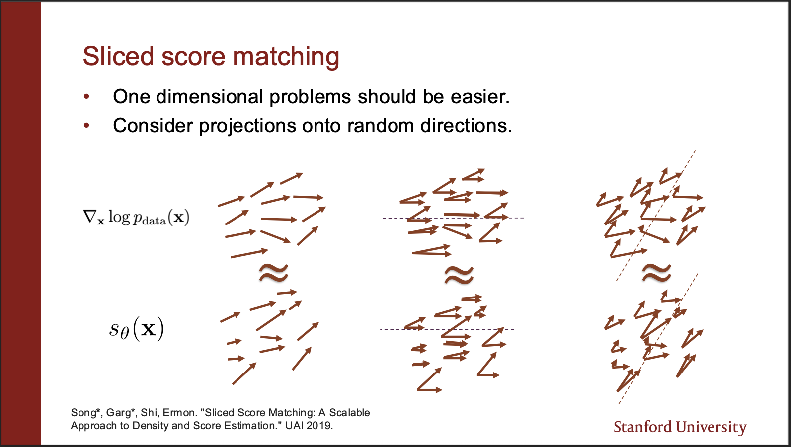
There is another algorithm called the sliced score matching. So consider a vector field of $p_{data}$ which is very high dimensional. So we can imagine that we can `project’ those vectors to some lower dimensions. The distance estimation on a set of vectors then reduces to distance estimation on a line (Which is much more computationally efficient in practice. )

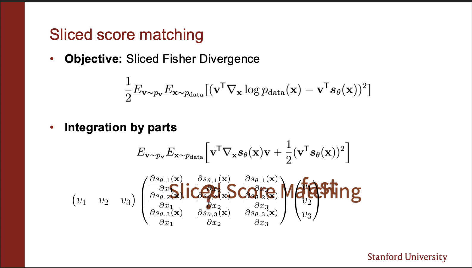
The score function can be modelled as a fisher divergence between the ground truth data, and score matching network. The key component in the equation is $v^{T}$ which projects the predicted vector field onto a straight line. Take a closer look at the second equation. It consists of $v^{T}\nabla_x v.$. Mathematically, it means that the jacobian (the two dimensional matrix) , is multiplied by a same vector, and its transpose on the same end. The final value is a scalar. Now, the key idea is that this ‘weird product’ is somehow much more efficient to compute. How?

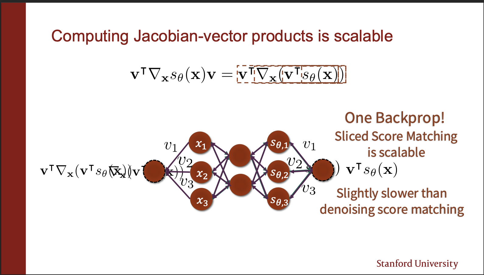
Because it can be modelled as a single backprop step? How? Take the output of your score network, take a dot product w.r.t $v^{T}$, backpropogate, and take another dot product w.r.t $v^{T}$ again!!. So, you no longer have to take $d$ products, where d is the number of input dimensions!!. This makes the learning process much more stable in practice.

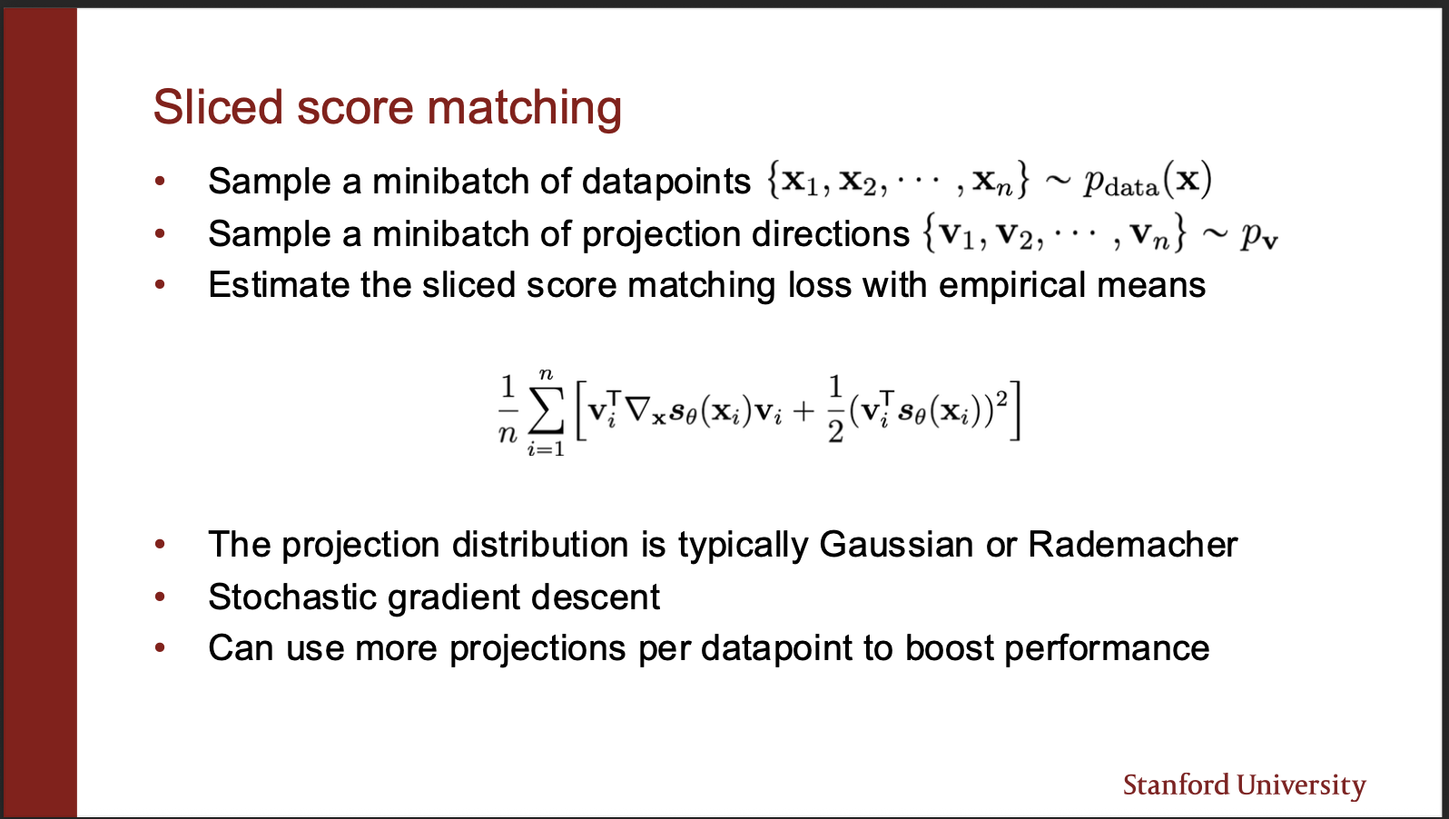
So the algorithm of sliced score matching becomes simple, take input images, generate random projection directions, compute the weird derivative, backpropogate. so remember their are two backward passes in this algorithm 1) where outputs of score network are multiplied w.r.t v, here the aim is not the optimize the parameters. 2) actually updating the parameters of the network. One argument may be: how to choose this projection direction $v$. Note that we are sampling those directions randomly, so even if “loss of information” happens while projecting the outputs of score network, the fact we sample “random” projection directions, more than compensates for it. What we lose, is what we gain in efficiency, just 2 backprops per forward passes.

So we have discussed how to ‘train’ sliced-score-matching network. How to sample from it?

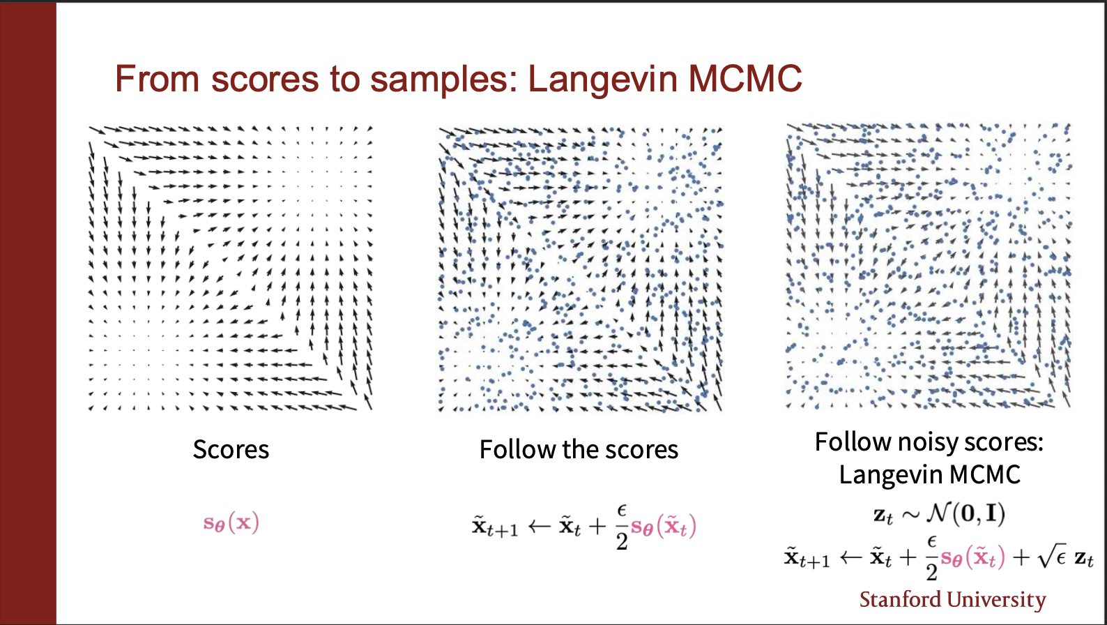
We can use normal langavian dynamics idea: choose a random starting point, take a step along score function, sprinkle a little bit of gaussian noise, to get a variety of samples in the generation process.

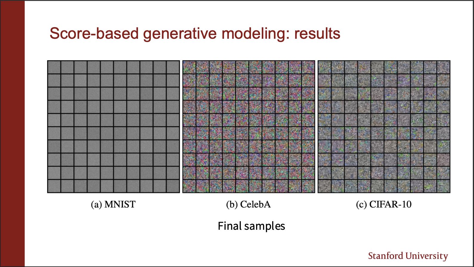
Following this algorithm, however DOES not work, all it gives us is this blurry samples, which make no sense. Alas!!, what is the use of so much math, if it doesnt work. Fortunately, there are two subtle reasons for this problem:

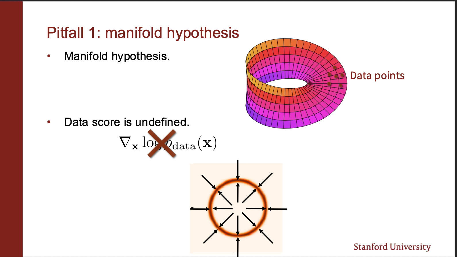
This is the manifold hypothesis. Your data lies only on a manifold of a high dimension space. If you initialize the starting point of your sampling algorithm in some empty space, the gradient field is undefined!!. Its like you are standing in land, and cant navigate to different points in the river.

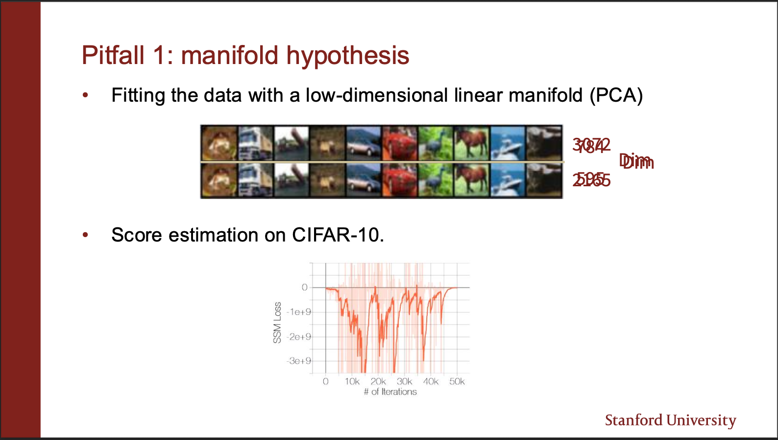
Lets say the representation of our image lies on a 3072 dimensional vector spaec. If you reduce its dimension, to 2056, turns out, the image can still be perfectly reconstructed. This means, that “most of the space” in the high dimensions is empty.

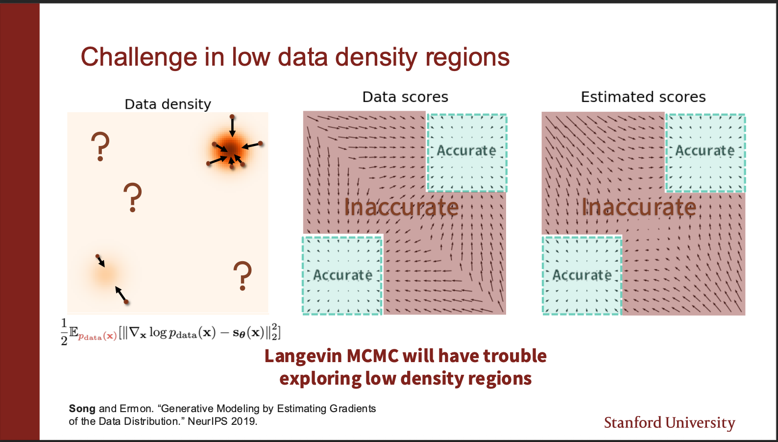
An intuitive insight goes as follows. On the left, we show a data distribution consisting of two gaussians. The data density in top left, and bottom right region is really ‘low’. If we look at the score function in the red region, it turns out that it is pretty inaccurate, whereas only the green regions are accurate. So, if you initialize your starting point in red region, there are chances you will just keep roaming around in the red regions, and never actually end up in the green region. And all you will see is noise.

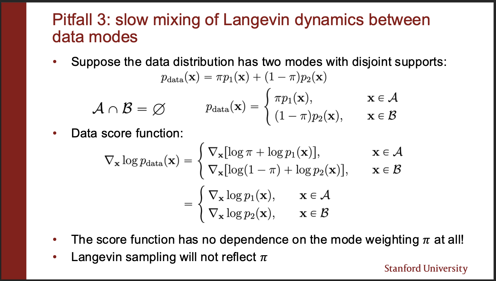
Another problem goes as follows: Suppose you are given a mixture of gaussians which mix information in “different weights”, for eg, $\pi$ amount from gaussian A, $1-\pi$ amount from gaussian B. The constraint is that a particular sample $x$, can only belong to either A or B (disjoint mode). When you model the score field of such a mixture i.e. the gradient, instead of actual likelihood (i.e. $p_{data}$), you lose the coefficients!!.

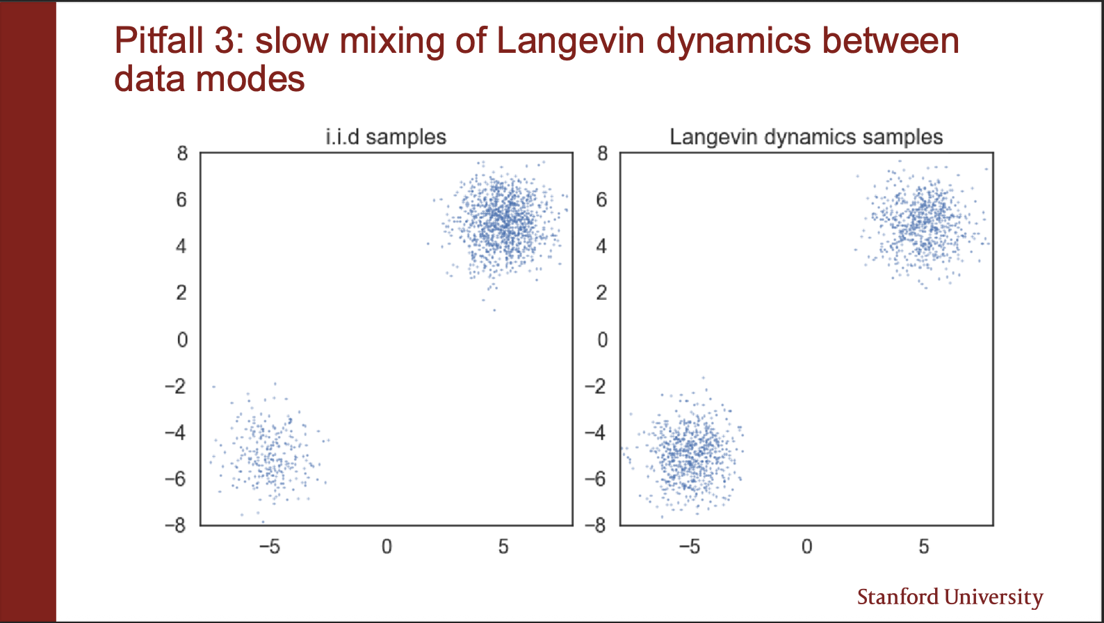
On the left we show “unequal samples distribution”. i.e. there are less samples in the bottom left gaussian, and more samples in the top right gaussian. However, when you build a score function, and then sample the points, you will see that they generate “equal densities”. As seen in the right figure. However, this is not correct.

Now, you “somehow” fix these issues, and you will be able to generate cool looking samples like the above photo. The fixes will be discussed in a later post.

———–Approaching the end of this post——–

Woah, so much math. OMG. If you got through it, you are a superhuman (really). I know you don’t like math. I also dont like it. Hell i dont even understand it. But hey, here is the kicker: There is more math coming :-)!! We will talk about the supercool diffusion models in the next post.

It is very easy to listen to a lecture and then make notes. But what is difficult is making the inutuition clear to others. I could definitely have not gained this depth by reading papers, merely watching lectures: because i don’t know the broader field history. Neither do i know, in what orders to read papers in. Conferences have become huge: most papers are trash (even mine)!!. That is where the classroom programs come in handy. I just wish my own school (UCF) had such deep lectures :-). Thanks to stanford for making their amazing content available to us ‘common’ men. That is the reason for writing this blog: it benefits ME (because i’m selfhish :-)). But, if it benefits you too, i’m grateful.

rajat