[Part 1: Object Detection] [RCNN] On the internal mechanics of Region Proposal Networks.

Says Lord Krishna to Arjuna: One should engage oneself in the practice of yoga with determination and faith and not be deviated from the path. One should abandon, without exception, all material desires born of mental speculation and thus control all the senses on all sides by the mind. - Srimad Bhagavad Gita

The eight limbs of yoga or “ashtang” as it is properly called form the crux of Patanjali’s teaching. Like all the great arts, the underlying tenets of machine learning algorithms lie in Image Classification. How is a CNN able to look at an image and output a single value resembling the probability of a class to which an image belongs? Imagine for a moment that you are a neural network. The user gives you a 3-channel image matrix containing random numbers. You have to compress this 2D matrix into a single value. But, what is the deeper level of operation other than our current understanding that a CNN learns random filters through a cascade of non-linear layers & applies a soft-max unit in the end for performing classification?

Among us nerdy folks, a simple experiment amazed us. Consider an image containing a single cat. Your network outputs a certain value (say 0.7) which corresponds to the probability of the cat being in the image. During the inference phase of our classification model, we rotated the cat and observed the fluctuations in the confidence scores. It isn’t 0.7 every time which showed us that the CNNs are not that much scale/rotational invariant as others claim them to be. If you increase the number of cats in the image, the confidence value of the network increases. If a single cat is gradually phased out of the image, the classification score drops. Behind the single number (0.7) which we observe, the network actually learns where the object classes lie and internal activations perturb proportionally to multiple instances of the same class.

Training the network on classification task, performs internal localization of the object instances present in the image. A very valid question thus becomes if the features learnt on classification models can be transferred to the detection based tasks. Perception occurs along 5 stages, each of which form a core component of a machine learning pipeline.

1. Classification: Gives a global context to the network about the type of objects present in the image. For eg, an image contains the cat, dogs etc.
2. Localization: The filter of a CNN layer becomes sensitive to presence of a particular class. Magnitude of activation acts as a rough attention based mechanism as to where an object might be.
3. Detection: After zoning in on a pattern on activation, a precise geometrical inference is made about the object location. This is most popularly understood as the task of outputting bounding box around an object.
4. Recognition: Among successful detections of the same class, the network learns to separate multiple instances of the same class.
5. Tracking: The final task requires us to track the object over a sequence of frames (By assigning an object id) and maintaining a sense of its trajectory.

In this post, we are gonna be focusing explicitly on the detection task and understand how our existing knowledge of image classification helps us to naturally build object detectors. For the moment, we are gonna consider something very trivial and consider build from there.Suppose we want to detect the exact location in an image where a cat is present. If, there had been no CNN’s, what will be the approach to detect such a cat?. The traditional methods would have taken two steps:

1. Find the interesting regions in the images where a cat might lie.

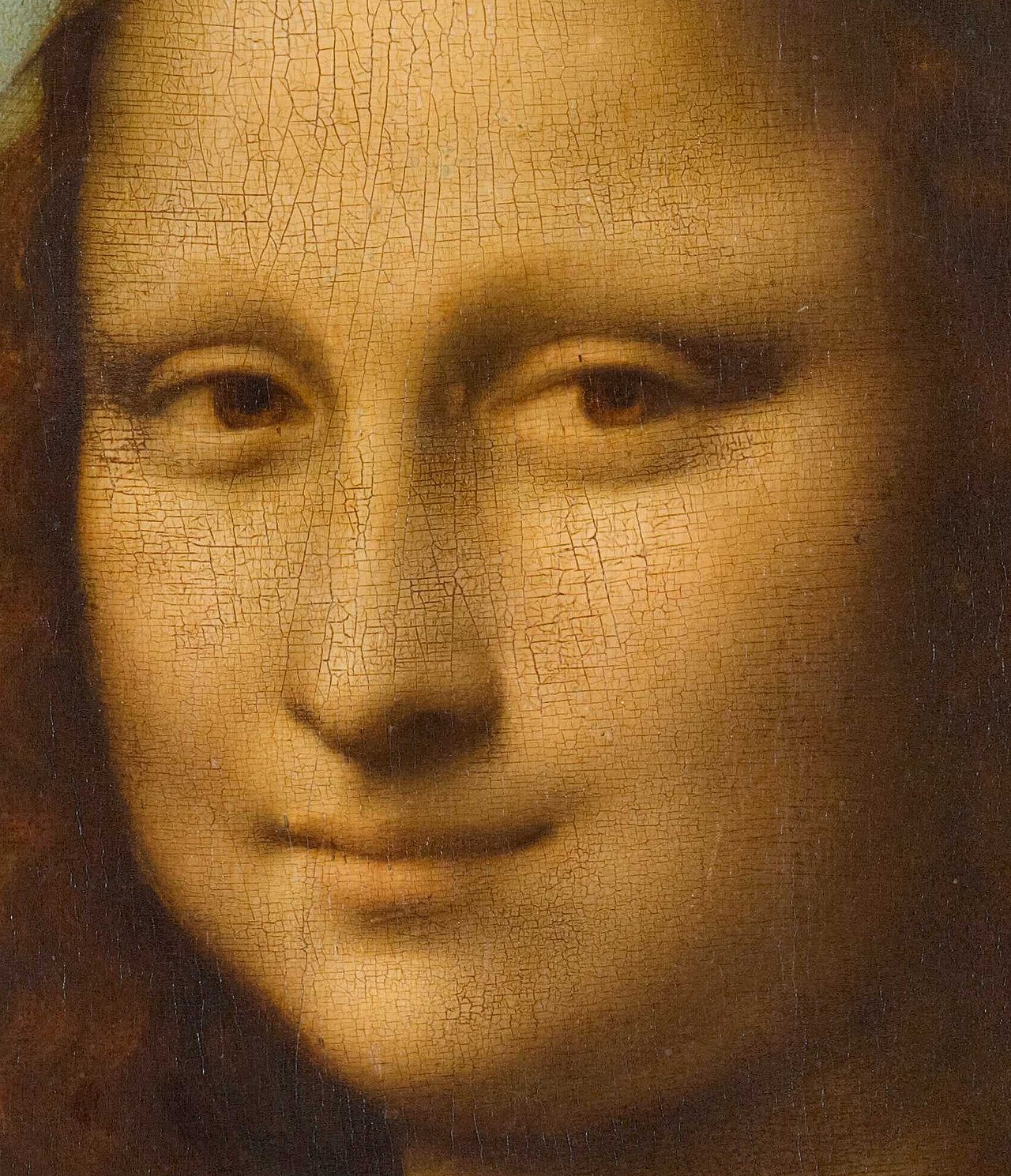
The best way to isolate objects in an image is to identify their boundaries. Traditional detectors like canny & HOG would have operated on the gradient change in the pixel intensity values to filter individual object identities . However, Da-Vinci explained a fundamental point in his paintings that the objects don’t hold fine boundaries in real world. Instead, the object boundaries gradually merge in their backgrounds via the sfmato effect.

1. Compare the object boundaries to find similar objects The boundary [skeleton] of the cat obtained in the previous step would have been compared with the skeletons of cats already known. If they match, then it is a positive detection. But there are several questions that trouble us. Does a cat hold same skeleton across many frames? No, because the cat might change its pose, orientation. Similarly, can multiple animals hold same skeleton?. It is possible. This phenomenon leads us to conclude that:

• It is impossible to determine the identities of multiple objects by only examining the contents of their boundaries. Instead, we need to devise mechanisms that examine the contents inside these boundaries also. (Identically sized dog and cat possess same boundary, but different internal structure).

• A single object can hold the boundaries of different dimensions (a cat can change its pose). There is no way via which we can converge onto single boundary of an object due to this dynamic constraint.

Therefore, our machine needs to perform detection on two granularities. Firstly, it needs to combine the notion of object boundaries (localization) with the contents inside boundary (internal representations) to obtain an object representation at a single parameter (which can be the pose of a cat). Then, it needs to map multiple such representations to a single representation that is invariant to the transformations in the cat’s structure. Only when the above two steps are achieved, can the identity of a “cat” be compared with the identity of a “dog” class, to differentiate amongst objects of multiple classes.

With such semantics in place, let’s return to the task of detecting cat in the image. We already possess the capability to answer the question whether an image contains a cat or not. (the naive classification task). Can this be used to perform detection? We could partition our image into smaller regions and check whether each of these regions contains a cat or not. Partitioning a larger image into smaller chunks is gonna face several issues:

• Large number of chunks- As the height/width of the cat image increases, the number of chunks which we end up creating will increase.
• The scaling issue- We don’t know how much should be the size of the chunk we create. In case the cat in the image is larger that our chunk, we would need to combine several chunks together to find the final coordinates of cat in the image. This phenomenon is known as LANMS (but is typically used in the end stages of Object detection models, not the beginning)

So, it seems that image classification can help us perform object detection. But, we would need to solve the computational constraints that our approach of classifying each chunk we partition our image into faces. Furthermore, we are still not confident whether the chunks we should create should be of identical sizes since a same cat might be of many different sizes in an image. So, we ask a more fundamental question? Provided we accurately find a single chunk that surrounds a cat, can an Image classification model detect whether that chunk contains a cat? The answer is Yes. This means that our detection system should have a notion of precise detection followed by an Image classification network. But, there is going to pose a more fundamental problem.

Our discussion had started with the fact that image classification might lead to object detection. But, in the previous paragraph we arrived at the fact that we need to perform accurate detection first (accurately choosing a feasible chunk) and then image classification. These two statements contradict each other as to which of the image classification or chunk localisation should occur first in an object detection machine. The answer lies in realising the following fact:

• We cannot perform detection efficiently without performing image classification first. But our approach of trying to choose a precise chunk (i.e. trying to find a precise chunk that surrounds a cat properly) before predicting whether it contained a cat/or not was wrong.

The best we can do is to find some rough chunks that may surround a cat, classify them and look at their confidence scores on Image classification models. And among those guys where confidence score is high, we can try to refine our chunks coordinates later. This helps us to devise the fact that our detection pipeline should consist of rough chunk localisation, image classification and iterative chunk refinement as its cascaded components. This is the fundamental concept behind RCNN.

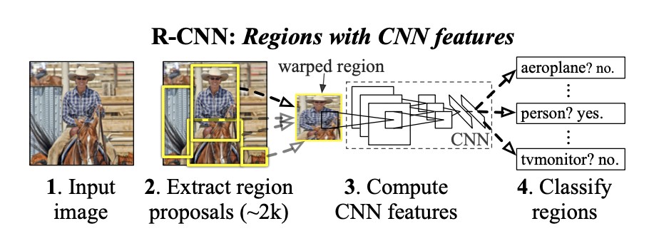
There is a grand beauty to the architectural flow we show above.

1. Region Proposal [Rough Chunk Localisation]: Based on our discussions, the first step has to be to partition the image into rough chunks that might contain an object. This is achieved by using traditional computer vision approaches. The important point to note is the number of chunks we actually require to predict. Another important question to ponder upon is about the size of the object inside each chunk. We shall skip the first question for now. Each chunk (rectangle) we create in the figure above can be of different size. But, a CNN requires a fixed sized input to operate as per our current understanding. So, we need a mechanism to compress chunks of different sizes into identically sized input. This is achieved by warping the chunk inputs. The major disadvantage of this approach is that the relative aspect ratio (height:width) of the object gets distorted. CNN’s are not distortion invariant by design. So, the fundamental problem in RCNN is it’s tendency to warp each of the chunks to identically sized input.

2. Region Classification [Image classification]: In the above step, we asked our machine about the possible regions which might contain a cat. It spits out some fixed number of proposals (say 2000) which might contain a cat. As discussed before, the next task is to check whether any of these proposals actually contains a cat or not. So, what will we do. We will take a rectangular chunk, warp it into fixed sized input and pass it through an image classification model. At the output end, we would look at it’s confidence score. The important point to understand here is how many forward passes do we have to make through our CNN in this case? We would say 2000, since we are asking the question of whether a cat is present or not for each chunk we create. This means that I cannot definitely isolate the region where a cat is present till the time all the chunks make a forward pass. This leads us to understand that RCNN’s limitation is the fact that it needs to make multiple forward passes for each of the region proposals it creates. Since, each of the region proposal is of the same size (due to so called warping), we could have concatenated all the ROI proposals along the batch dimension of the input and made a single forward pass. But, the problem is that traditional batch creation requires concatenating “contents of multiple samples together” & not the “contents of a single sample”. If I try to concatenate 2000 ROI proposals of image 1 along with 2000 ROI proposals of Image 2, we would need to limit the number “2000” for each of the image we operate upon. But, an image might not contain 2000 proposals everytime. So, this means that to devise our machine we need to solve three problems:

• What is the method through which forward passes for multiple chunks can be made at a single time.
• We discussed that 2000 chunks cannot be concatenated along channel dimension. So, How do we compress these 2000 chunks into a single representation?
• From a single representation that a CNN outputs, how do we reconstruct the identities of the 2000 chunks together? A critic might ask us what is the need to reconstruct the chunks together. We shall endeavour to answer this in the upcoming paragraph.

1. Classification: So, we have computed the confidence scores for each of our proposals. Till now, our limitation had been thinking that a proposal might contain a cat only. But, It might contain multiple classes. So, a more valid question to ask is “what class does a particular chunk belong to”. This means that we need a classifier for each of the class. So, if we need to ask ourselves whether a chunk belongs to 5 classes, we need 5 classifiers. This will create a further problem. Our CNN will output 2000 candidate regions. Each of these regions might belong to one of 5 classes. If, we want to simultaneously predict the classes to which each of these regions might belong to, we would need 20005=10000 classifiers. If we increase the number of candidate proposals (from 2000 to 3000), we would end up needing 30005=15000 classifiers. This is an impossible task. So, how do we solve this problem? What we can do is come back to our trusted old image classification. Treat 2000 candidate proposals as 2000 separate images. So, we have 5 classifiers for each class. For each candidate proposal, we try to classify the class it belongs to by using the same 5 classifiers. But, 15000 classifiers were capable of predicting classes in a single shot. If we try to reduce them to 5 classifiers, we will have to wait till each of the 2000 proposals gets classified. RCNN does not solve this problem. It keeps 5 classifiers, and waits till all the 2000 proposals give their class predictions.

There is one more problem. To train a classifier we need data. Our need is to devise a classifier that can look at a candidate proposal and tell if it contains a cat or not. So, if our dataset contains 1000 images & 2000 proposals for each image, then 2k*1K= 2e-6 proposals will have to be stored in the disk before our classifier can be trained. This illustrates the fundamental problem in RCNN that prevents it to function as a single e2e trainable model.

1. All the proposals or CNN outputs are stored in disk . Classifiers (like SVM) are separately trained.

2. The CNN is first trained, and then the classifiers. This prevents the network to train end to end.

Once the candidate proposals are assigned to their respective classes, we need to adjust them slightly to compensate for the rough region proposal we made earlier. This is achieved by the bounding box regressors, which was not a part of the v1 RCNN paper. We will explain more of this in the next post. For now, the important thing to realise is that although RCNN manages to introduce Deep CNNs to the context of object detection, they face the problems of input warping, predicting fixed number of proposals, and training separate classifiers that requires large disk space (to store candidates). Some of these problems have been solved in the later variant SPPNET which we shall focus more on later.

rajat